Tutorial 2 — A geospatial flow map on a globe
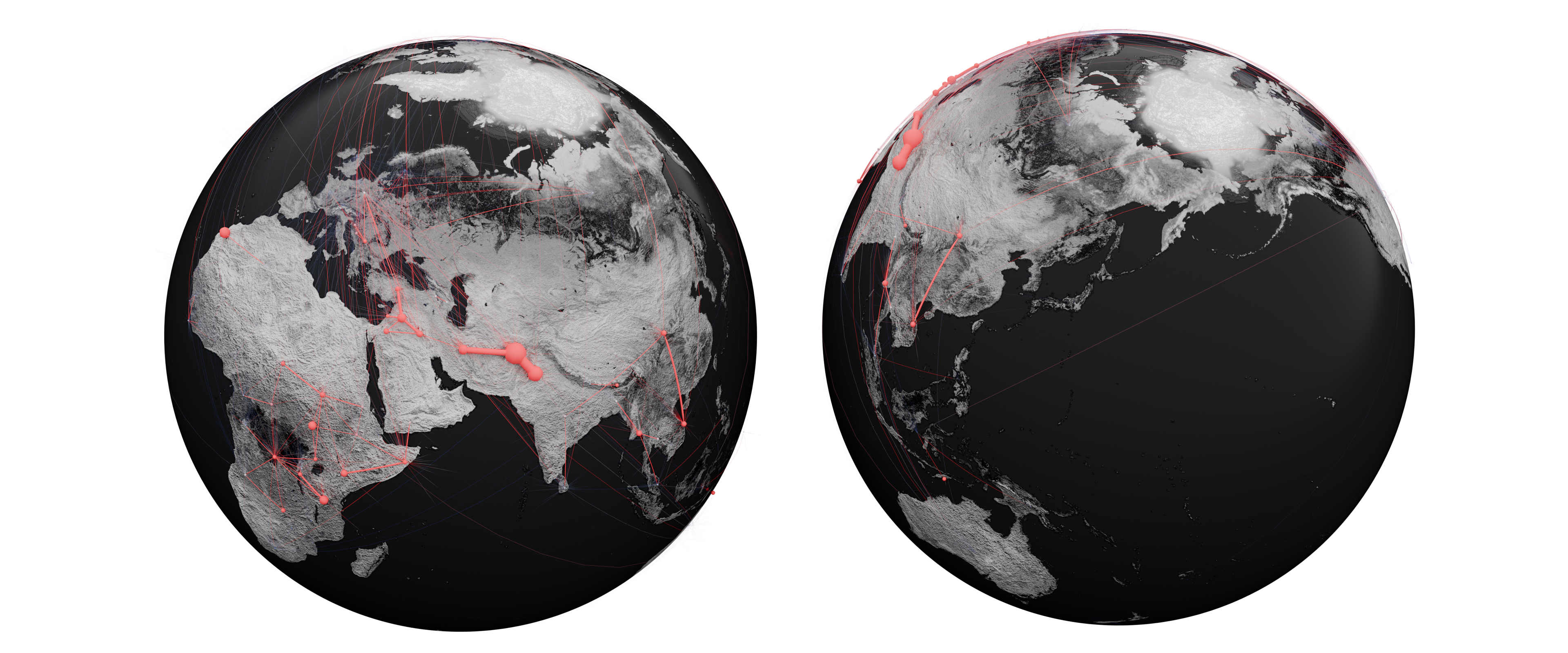
Reproduce the kind of global flow map shown in the SciGraphs paper: nodes are countries placed on a 3D globe, edges are geodesic great-circle arcs, and node size encodes a flow volume.
What you need: an edge list whose source/target columns are place names (countries or cities), ideally with a weight column for flow volume — or explicit latitude/longitude columns.
1. Import with geocoding
- Open SciGraphs ▸ Data and load your file (File source, set the delimiter, Load File).
- Map Source Nodes / Target Nodes and set the Weight Column to your flow volume. Enable Directed Graph if the flows are directional.
2. Configure the globe
- Expand the Geospatial Options subpanel and enable it via its header checkbox.
- Turn on Auto-Geocode Source/Target as Countries/Cities so the node names are resolved to coordinates via Nominatim. (Alternatively, disable geocoding and point the Latitude/Longitude fields at coordinate columns.)
- Enable Show Earth Globe, set the Globe Radius and Globe Quality.
- Choose a Globe Theme — e.g. NASA Blue Marble for satellite imagery — and tune the PBR Settings (water shine/roughness, land roughness, surface relief). Use Pre-download to cache the texture.
- Set the Edge Style for the geodesic arcs.
3. Create the graph
Press Create Graph in Step 3, then Setup Visual in Step 4. The nodes are placed on the globe and edges are drawn as great-circle arcs.
In geospatial mode the layout step is skipped automatically — positions come from coordinates, not from a layout algorithm.
4. Encode flow volume
- In Visualization ▸ Appearance, drive node size from the weighted in-degree (total displaced population) using the attribute multiplier.
- Colour nodes or arcs by origin/destination class or by volume with a scientific colormap.
5. Render
Frame the globe with the camera, add the lighting rig (Scene Setup), and render with Cycles for path-traced imagery. Because the graph attributes (flow volumes, classifications) remain accessible, you can re-style interactively without re-projecting.
This workflow produces publication-quality imagery that is impractical to achieve in conventional 2D network tools without exporting geometry to external 3D software.