Tutorial 4 — A sparse matrix from SuiteSparse
Import a benchmark matrix from the SuiteSparse Matrix Collection, lay it out (or use its intrinsic coordinates), and colour it by eigenvector centrality — the recipe behind the sparse-matrix gallery in the SciGraphs paper.
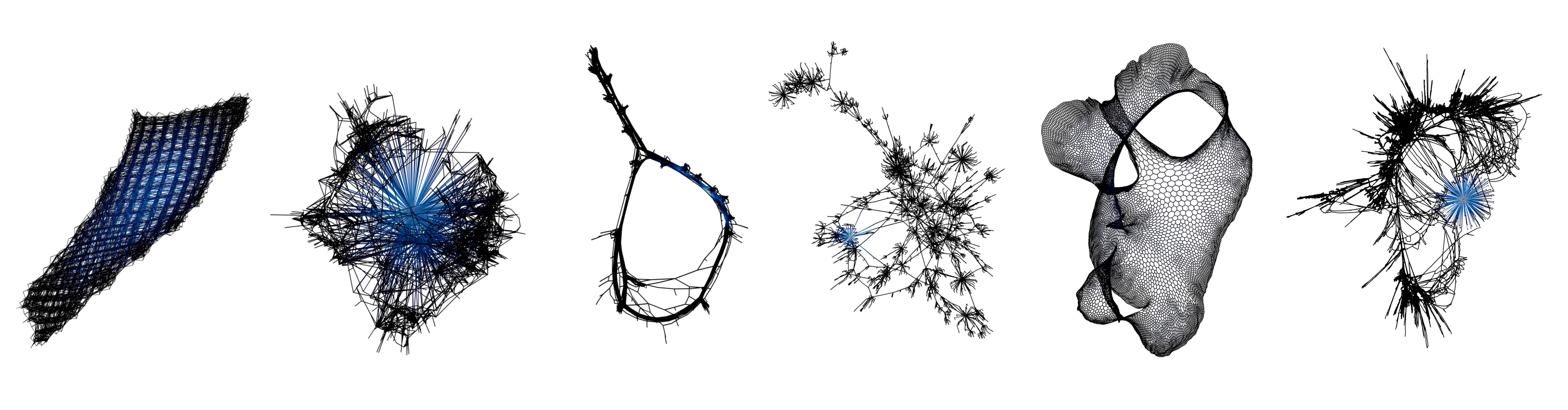
The SuiteSparse Matrix Collection contains over 2,800 sparse matrices from real-world applications (finite-element meshes, circuit simulations, optimization problems, and more), making it an excellent benchmark corpus.
1. Import a matrix
- Open SciGraphs ▸ Data and set the source to SuiteSparse.
- Enter a Matrix Identifier in
Group/Nameform (e.g.Grund/bayer09). Use Browse Collection to find identifiers. - Choose the Graph Representation:
- Symmetric — interprets the matrix as a standard adjacency graph via \(A + A^\top\) (denser, rounder layouts).
- Bipartite — treats rows and columns as two disjoint node sets, preserving the original matrix structure (elongated layouts).
- Enable Giant component only to keep just the largest connected component.
- Optionally enable Auto layout on import and pick Yifan Hu as the default layout.
- Press Download & Create Graph.
If the archive ships an auxiliary coordinate file, SciGraphs applies those coordinates directly as vertex positions and skips the layout entirely, faithfully reproducing the geometry of the underlying physical domain.
2. Lay out (matrices without coordinates)
For matrices without coordinate data, open Layout & Positioning and apply Yifan Hu (sfdp) in 3D — it typically produces the most informative results for large sparse structures.
3. Colour by eigenvector centrality
- Run Setup Visual (Data panel, Step 4) if you have not already.
- In Analysis ▸ Centrality Metrics, choose eigenvector and press Calculate.
- In the Visualization panel, map node colour to the eigenvector-centrality attribute using a colormap such as Inferno or Black-Body Radiation. Bright nodes mark the vertices most central to the dominant eigenstructure; dark regions are peripheral.
4. Render
Add lighting and a camera, then render with Cycles. For dense meshes, depth of field and adaptive text labels (label only high-degree nodes via the Attribute Filter) reduce visual clutter and reinforce depth perception.
Building a gallery
Repeat the import for several identifiers spanning different problem domains to assemble a morphological gallery, then arrange the resulting objects in a single scene for a comparative figure.