Tutorial 5: A reproducible pipeline
A pipeline specification is a JSON or YAML file with one block per stage of the workflow: dataset, analysis, layout, styling, lighting, labels, render and export. Running it reproduces the whole figure, since the same seed and the same inputs give the same result on any machine with the add-on installed. Each run also writes a manifest recording the versions it used and a SHA-256 for every file it produced, so a third party can check that they got what you got.
Ready-to-run specifications
Each specification below is complete and produces the figure shown beside it with no editing.
Download one, then drag it from your file manager onto the 3D Viewport. With SciGraphs enabled it runs immediately, writing its outputs and a provenance manifest beside the file.
You can also set the Pipeline file in SciGraphs ▸ Reproducibility and press Validate, then Run.
From a terminal, without opening Blender
This runs a specification headlessly and needs nothing but Blender with SciGraphs installed:
blender -b --python-expr "import bpy; bpy.ops.scigraphs.run_pipeline(filepath='/path/to/spec.json')"Outputs and the manifest land beside the specification as they would from the interface. Progress goes to stdout, prefixed [SciGraphs Repro].
For scripting or continuous integration, exit on the operator’s result so a failure stops the build instead of passing silently:
blender -b --python-expr "import bpy, sys; sys.exit(0 if 'FINISHED' in bpy.ops.scigraphs.run_pipeline(filepath=sys.argv[-1]) else 1)" -- /path/to/spec.jsonBlender itself exits 0 whatever happens inside the script, so the sys.exit is what makes a broken specification visible. Everything after -- is passed to the script rather than interpreted by Blender. To regenerate a set of figures, loop over the specifications and compare each manifest’s digests against the ones recorded previously.
Paths beginning // resolve against the folder holding the specification, so keep a downloaded file next to any data it references. Two of these download a street network live from OpenStreetMap; the rest need no network.
Les Misérables from a GEXF file
Rank normalization on a betweenness distribution that is half zeros
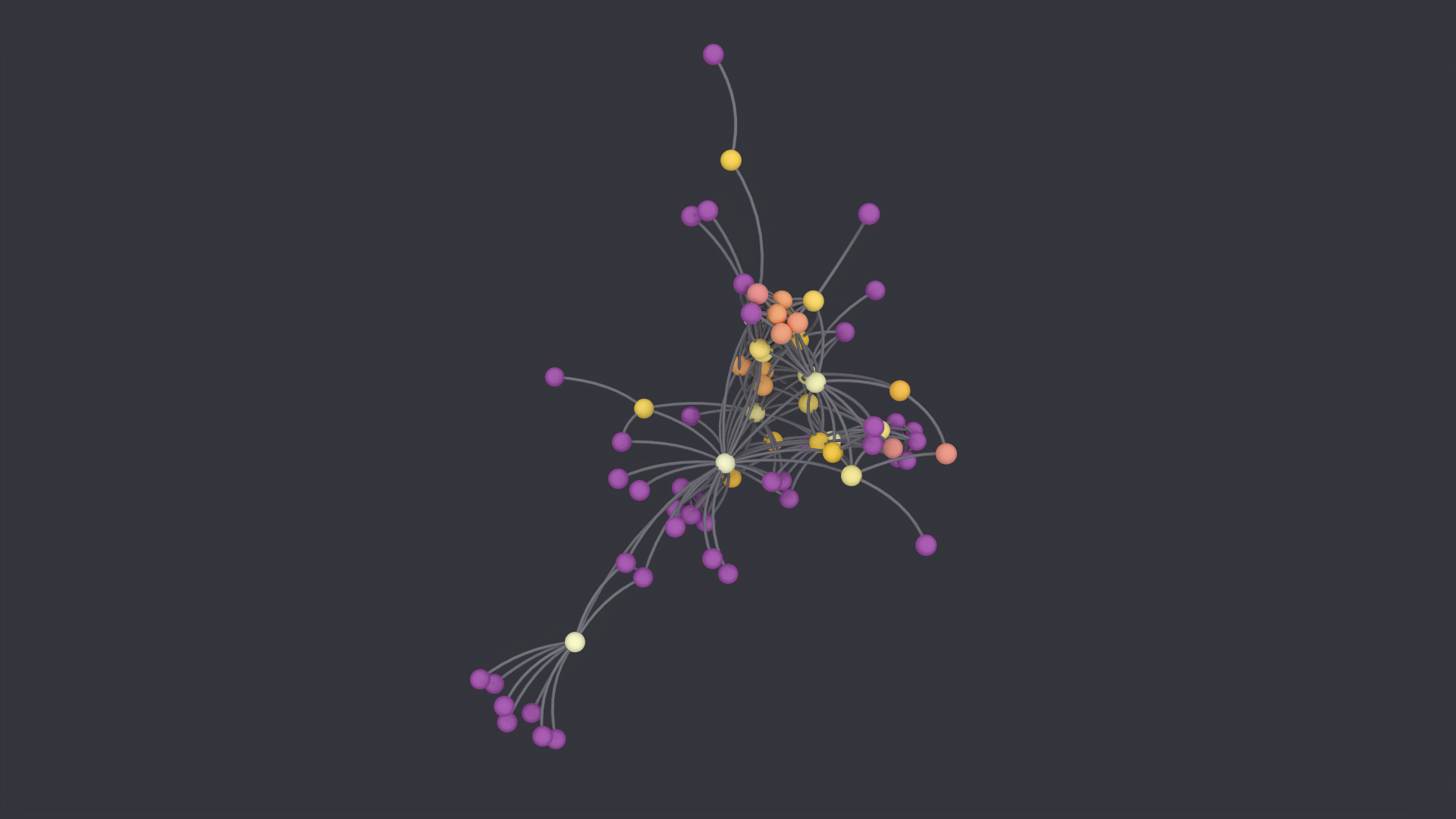
The co-appearance network of Les Misérables: 77 characters, 254 edges, distributed with the specification so the example runs with no network access.
Betweenness here is extreme even by the standards of social networks. 43 of the 77 characters have betweenness exactly zero, appearing only alongside someone more central, and the maximum, Valjean, reaches 0.57. Normalized linearly onto a colormap, 71 of 77 nodes fall in the lowest tenth and only 5 of 10 color bins are used at all.
color_norm: RANK replaces each value by its position in the sorted order. The bins become 8, 8, 7, 8, 7, 8, 8, 7, 8, 8, uniform by construction. The limit is visible too: the 43 tied zeros share one rank, so they share one color. Ranking fixes the distribution, not the ties.
| Source | gexf: lesmiserables.gexf |
| Engine | Cycles |
| Color transform | RANK |
| Metrics | degree, betweenness |
| Sections | meta · dataset · analysis · layout · visual · world · lighting · render · exports |
fig1_flatfile_lesmiserables.json
{
  "meta": {
    "title": "fig1_flatfile_lesmiserables",
    "seed": 42,
    "output_dir": "//repro/fig1_flatfile",
    "description": "Flat-file ingestion (GEXF). Demonstrates rank normalization: betweenness on this graph is heavy-tailed, and a linear ramp would put almost every node in the darkest color.",
    "clear_scene": true
  },
  "dataset": {
    "source": "gexf",
    "filepath": "//data/lesmiserables.gexf",
    "auto_layout": false
  },
  "analysis": {
    "metrics": [
      "degree",
      "betweenness"
    ]
  },
  "layout": {
    "algorithm": "SPRING_3D",
    "scale": 5.0,
    "iterations": 150
  },
  "visual": {
    "setup_geometry_nodes": true,
    "node_color": "betweenness",
    "colormap": "inferno",
    "color_norm": "RANK",
    "node_glyph": "ICOSPHERE",
    "node_resolution": 24,
    "node_shade_smooth": true,
    "node_radius_rel": 0.022,
    "edge_radius_rel": 0.0035,
    "edge_resolution": 12,
    "edge_style": "CYTOSCAPE_BEZIER",
    "material_roughness": 0.35,
    "material_metallic": 0.0,
    "edge_base_color": [
      0.16,
      0.16,
      0.19,
      1.0
    ]
  },
  "world": {
    "color": [
      0.035,
      0.035,
      0.045
    ],
    "strength": 1.0
  },
  "lighting": {
    "sun_energy": 3.0,
    "sun_angle": 180.0,
    "replace": true
  },
  "render": {
    "engine": "CYCLES",
    "resolution": [
      1920,
      1080
    ],
    "samples": 96,
    "output": "figure.png",
    "denoise": true,
    "view_transform": "Standard",
    "filter_width": 1.0,
    "camera_lens": 60.0,
    "camera_margin": 1.12,
    "color_depth": "16"
  },
  "exports": {
    "positions": "positions.csv"
  }
}
Llíria street network, orthographic
Choosing a color transform by measuring what it does to the histogram
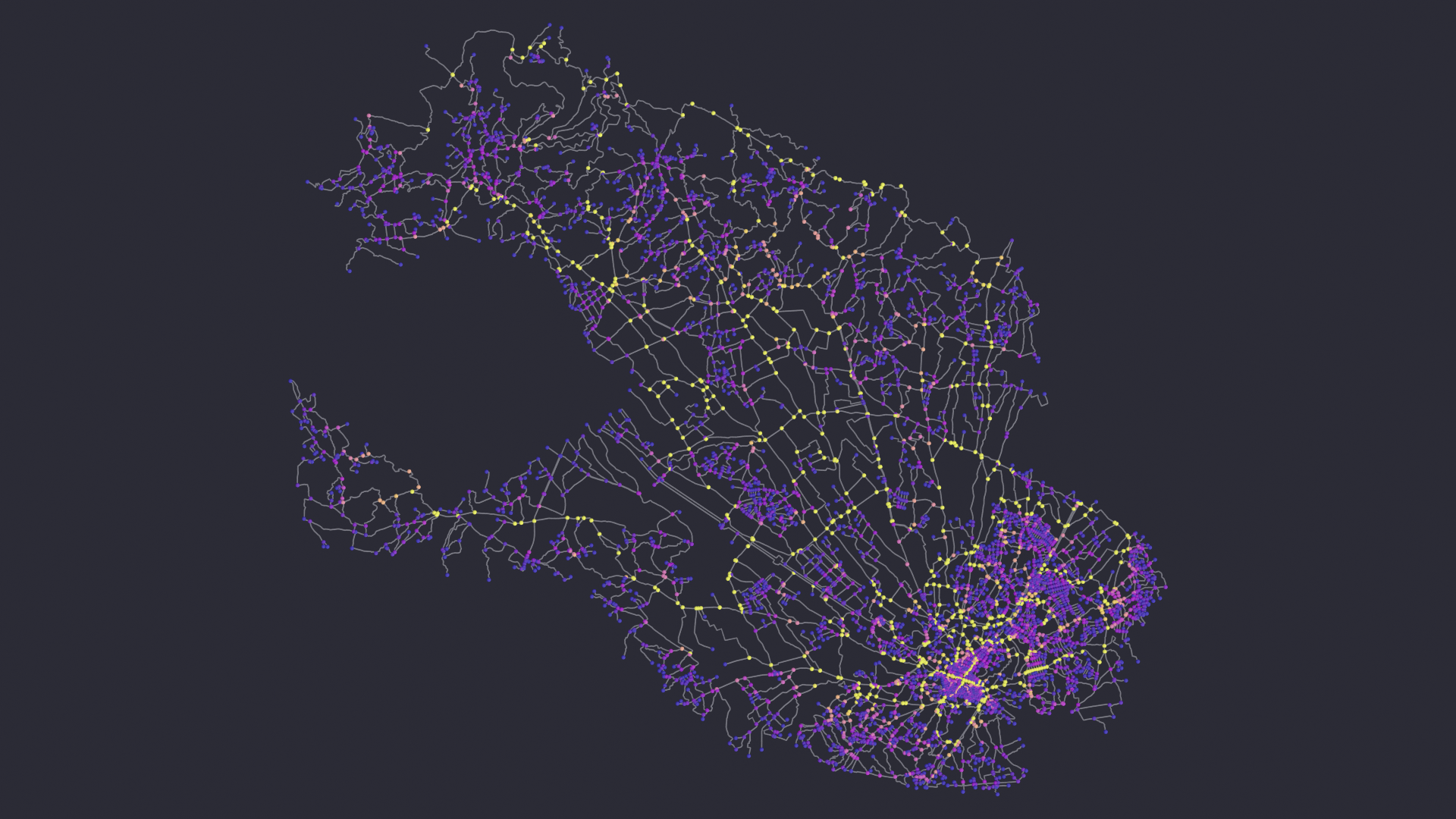
The walkable street network of Llíria (Valencia, about 23,000 inhabitants): 6037 nodes, 8067 edges, downloaded live from OpenStreetMap. There is no layout block on purpose. The coordinates arrive with the data, and a force-directed layout would discard the geography.
camera_ortho removes the near/far size falloff, so a node radius that encodes a value stays comparable anywhere in the frame. The cost is the loss of depth cues, a fair trade for a network that is essentially flat.
Betweenness here is extremely concentrated: median 0.001 against a maximum of 0.26, with 1112 nodes at exactly zero. How to map that onto a colormap can be measured rather than guessed. Counting how many nodes each transform sends into the brightest three tenths of the ramp:
color_norm |
Ramp bins used | Nodes in the brightest 30 % |
|---|---|---|
LINEAR |
9 of 10 | 8 (0.1 %) |
LINEAR, clipped at the 99th percentile |
10 of 10 | 159 (2.6 %) |
RANK |
10 of 10 | 1811 (30.0 %) |
LOG |
10 of 10 | 2419 (40.1 %) |
RANK and LOG both flood the image. They equalize the histogram, which is right for a graph whose ordering you want to read and wrong for one where the interesting fact is that a small minority of streets carry the through traffic. Plain LINEAR goes too far the other way: a single extreme node compresses everything else into one bin.
Clipping the top percentile and then mapping linearly keeps the concentration while spending the whole ramp. The arterial routes come out as continuous bright chains against a violet field, and their brightness still means magnitude rather than rank.
This example needs the Overpass API. When it is down, which happens, the dataset stage retries and appears to hang. Nominatim answering does not mean Overpass will.
| Source | osmnx: Llíria, Valencia, Spain |
| Engine | Cycles |
| Color transform | LINEAR |
| Metrics | degree, betweenness |
| Sections | meta · dataset · analysis · visual · world · lighting · render · exports |
fig2_osmnx_lliria.json
{
  "meta": {
    "title": "fig2_osmnx_lliria",
    "seed": 42,
    "output_dir": "//repro/fig2_osmnx_lliria",
    "description": "OSMnx ingestion. Ll\u00edria, Valencia (approx. 23,000 inhabitants). Orthographic projection, so node radius stays comparable across the frame instead of shrinking with distance.",
    "clear_scene": true
  },
  "dataset": {
    "source": "osmnx",
    "method": "PLACE",
    "query": "Ll\u00edria, Valencia, Spain",
    "network_type": "walk",
    "simplify": true,
    "cache": true
  },
  "analysis": {
    "metrics": [
      "degree",
      "betweenness"
    ]
  },
  "visual": {
    "setup_geometry_nodes": true,
    "node_color": "betweenness",
    "colormap": "plasma",
    "color_norm": "LINEAR",
    "node_glyph": "ICOSPHERE",
    "node_resolution": 16,
    "node_radius_rel": 0.0035,
    "edge_radius_rel": 0.0012,
    "edge_resolution": 8,
    "material_roughness": 0.4,
    "edge_base_color": [
      0.2,
      0.2,
      0.24,
      1.0
    ],
    "color_clip_percentile": [
      0.0,
      99.0
    ]
  },
  "world": {
    "color": [
      0.02,
      0.02,
      0.03
    ],
    "strength": 1.2
  },
  "lighting": {
    "sun_energy": 3.0,
    "sun_angle": 180.0,
    "replace": true
  },
  "render": {
    "engine": "CYCLES",
    "resolution": [
      1920,
      1080
    ],
    "samples": 64,
    "output": "figure.png",
    "denoise": true,
    "view_transform": "Standard",
    "filter_width": 1.0,
    "camera_ortho": true,
    "camera_direction": [
      0.0,
      -0.35,
      1.0
    ],
    "camera_margin": 1.06,
    "max_bounces": 4
  },
  "exports": {
    "statistics": "stats.json"
  }
}
A linear-programming matrix from SuiteSparse
A rectangular constraint matrix as a bipartite graph, laid out the way the collection lays out its own
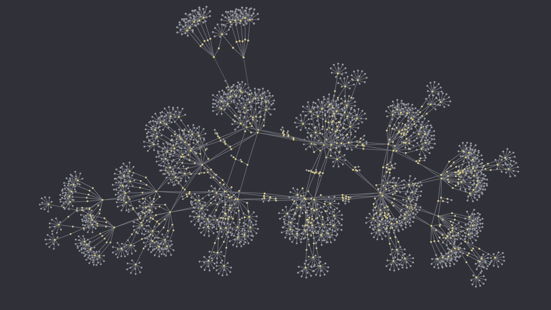
Meszaros/nemsafm is a linear program in standard form: 334 constraints by 2348 variables, 2826 nonzeros, 0.36 % dense. Read as a bipartite graph, one node per row, one per column, an edge per nonzero, that is 2682 nodes and 2826 edges.
The structure the drawing shows is in the statistics the run exports. Clustering coefficient is exactly 0, as it must be for a bipartite graph: no triangles. Median degree is 1 against a mean of 2.11, so most nodes are leaves; assortativity is -0.79, so those leaves hang off hubs. Together they produce the radial tufts. Diameter 22 over 2682 nodes gives the elongated shape, and the mean column degree of 1.20 says most variables appear in a single constraint.
The layout is YIFAN_HU, the multilevel force-directed method SuiteSparse itself uses for its gallery, so the drawing is comparable with the collection’s own. It places the graph in a plane with only slight relief, so camera_direction looks straight down that plane’s normal; the default oblique view would foreshorten it.
The matrix ships no coordinates, so a layout is required. In a structural mesh the auxiliary coordinate file is the embedding, and a layout would overwrite it.
| Source | suitesparse: Meszaros/nemsafm |
| Engine | Cycles |
| Color transform | RANK |
| Metrics | degree, betweenness |
| Sections | meta · dataset · analysis · layout · visual · world · lighting · render · exports |
fig3_suitesparse_nemsafm.json
{
  "meta": {
    "title": "fig3_suitesparse_nemsafm",
    "seed": 42,
    "output_dir": "//repro/fig3_suitesparse",
    "description": "SuiteSparse ingestion. A rectangular linear-programming constraint matrix read as a bipartite graph and laid out with the multilevel force-directed method the collection itself uses for its gallery.",
    "clear_scene": true
  },
  "dataset": {
    "source": "suitesparse",
    "matrix_name": "Meszaros/nemsafm"
  },
  "analysis": {
    "metrics": [
      "degree",
      "betweenness"
    ]
  },
  "layout": {
    "algorithm": "YIFAN_HU",
    "scale": 8.0,
    "iterations": 200
  },
  "visual": {
    "setup_geometry_nodes": true,
    "node_color": "degree",
    "colormap": "cividis",
    "color_norm": "RANK",
    "node_glyph": "ICOSPHERE",
    "node_resolution": 12,
    "node_radius_rel": 0.0035,
    "edge_radius_rel": 0.0011,
    "edge_resolution": 8,
    "material_roughness": 0.35,
    "edge_base_color": [
      0.2,
      0.2,
      0.24,
      1.0
    ]
  },
  "world": {
    "color": [
      0.03,
      0.03,
      0.04
    ],
    "strength": 1.0
  },
  "lighting": {
    "sun_energy": 3.0,
    "sun_angle": 180.0,
    "replace": true
  },
  "render": {
    "engine": "CYCLES",
    "resolution": [
      1920,
      1080
    ],
    "samples": 96,
    "output": "figure.png",
    "denoise": true,
    "view_transform": "Standard",
    "filter_width": 1.0,
    "camera_lens": 50.0,
    "camera_margin": 1.04,
    "camera_direction": [
      0.0,
      0.0,
      1.0
    ]
  },
  "exports": {
    "statistics": "stats.json"
  }
}
Xàtiva in EEVEE
The same specification on the real-time engine
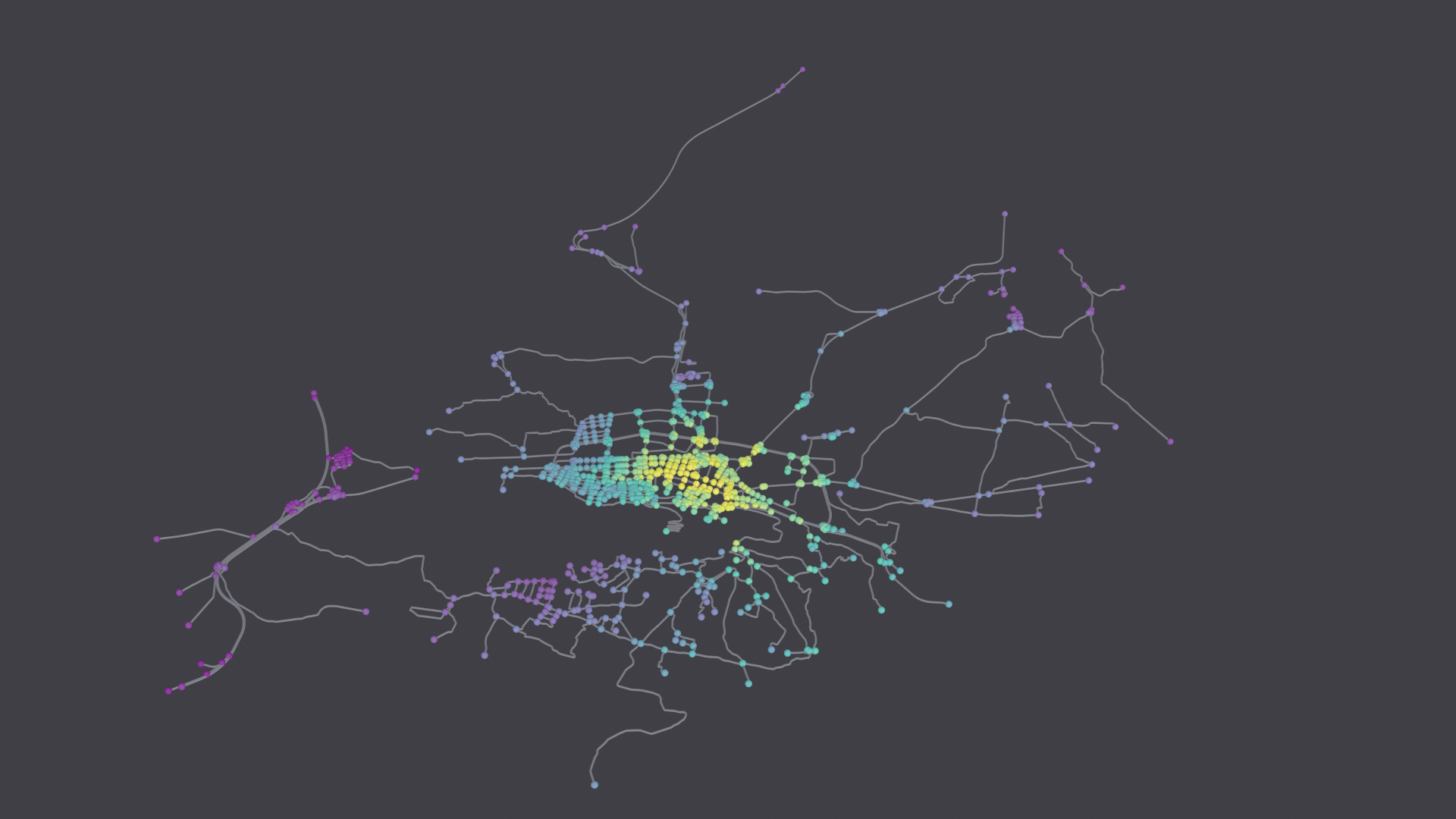
The drivable street network of Xàtiva (Valencia, about 29,000 inhabitants). Everything above the render block is engine-agnostic: the same dataset, analysis, color and glyph fields produce the same geometry, and only the last section differs from a Cycles specification.
Nodes are colored by closeness centrality under QUANTILE normalization, which ranks unique values rather than samples. That suits a grid-like street plan, which produces large groups of nodes with identical closeness.
ambient_occlusion darkens the crevices between clustered nodes, which lets a dense scatter read as depth rather than as a flat field.
| Source | osmnx: Xàtiva, Valencia, Spain |
| Engine | EEVEE Next |
| Color transform | QUANTILE |
| Metrics | degree, closeness |
| Sections | meta · dataset · analysis · visual · world · lighting · render · exports |
fig4_osmnx_xativa_eevee.json
{
  "meta": {
    "title": "fig4_osmnx_xativa_eevee",
    "seed": 42,
    "output_dir": "//repro/fig4_osmnx_xativa",
    "description": "OSMnx ingestion rendered with EEVEE Next rather than Cycles. Xativa, Valencia (approx. 29,000 inhabitants). Ambient occlusion is enabled through the ray tracing pipeline, which is what makes it take effect at all.",
    "clear_scene": true
  },
  "dataset": {
    "source": "osmnx",
    "method": "PLACE",
    "query": "X\u00e0tiva, Valencia, Spain",
    "network_type": "drive",
    "simplify": true,
    "cache": true
  },
  "analysis": {
    "metrics": [
      "degree",
      "closeness"
    ]
  },
  "visual": {
    "setup_geometry_nodes": true,
    "node_color": "closeness",
    "colormap": "viridis",
    "color_norm": "QUANTILE",
    "node_glyph": "SPHERE",
    "node_resolution": 14,
    "node_radius_rel": 0.005,
    "edge_radius_rel": 0.0016,
    "edge_resolution": 8,
    "material_roughness": 0.45,
    "edge_base_color": [
      0.22,
      0.22,
      0.26,
      1.0
    ]
  },
  "world": {
    "color": [
      0.05,
      0.05,
      0.06
    ],
    "strength": 1.0
  },
  "lighting": {
    "sun_energy": 3.0,
    "sun_angle": 180.0,
    "replace": true
  },
  "render": {
    "engine": "BLENDER_EEVEE",
    "resolution": [
      1920,
      1080
    ],
    "samples": 128,
    "output": "figure.png",
    "view_transform": "Standard",
    "filter_width": 1.0,
    "raytracing": true,
    "ambient_occlusion": true,
    "ao_distance": 2.0,
    "camera_direction": [
      0.3,
      -0.6,
      0.74
    ],
    "camera_margin": 1.08
  },
  "exports": {
    "statistics": "stats.json"
  }
}
Labeled characters
Ranking, occlusion and collision, in that order
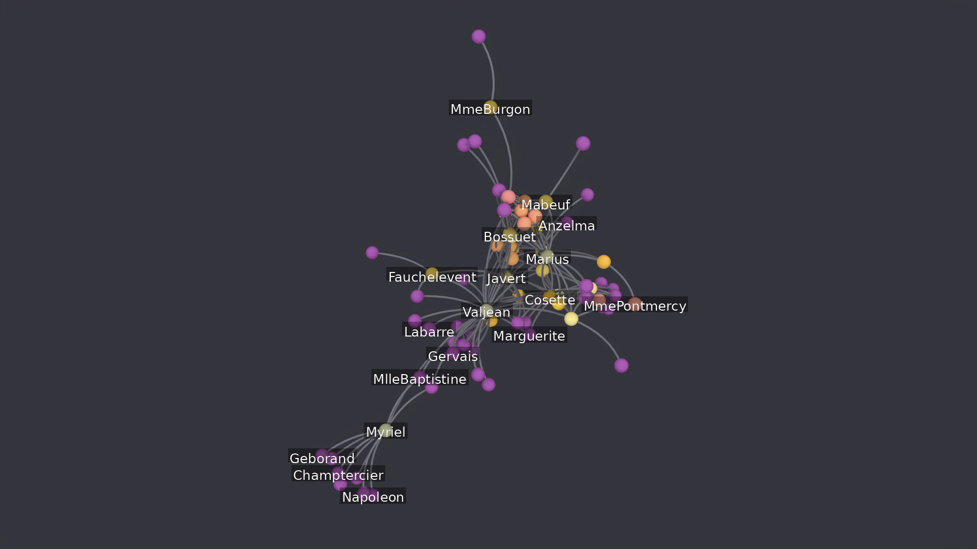
The same 77-node network with the eighteen highest-betweenness characters labeled.
Three filters run in sequence, and the run reports each: 77 nodes projected, 77 inside the frame, 59 not hidden behind geometry, 18 kept. rank_by decides the order, occlusion removes labels whose node is behind something, and declutter drops any label whose box would overlap one already placed.
max_count is preferable to a threshold. The centrality attributes are normalized to [0,1], so a cutoff calibrated on one graph means nothing on the next, whereas a count is bounded whatever the size or distribution.
| Source | gexf: lesmiserables.gexf |
| Engine | Cycles |
| Color transform | RANK |
| Metrics | degree, betweenness |
| Sections | meta · dataset · analysis · layout · visual · world · lighting · render · exports · labels |
fig6_labels_lesmiserables.json
{
  "meta": {
    "title": "fig6_labels_lesmiserables",
    "seed": 42,
    "output_dir": "//repro/fig6_labels",
    "description": "Node labels generated from a headless pipeline. The add-on's only entry point for this is an operator whose poll() rejects a background context, so labeled figures were unreachable from a specification; the underlying code never needed a GUI. Labels are ranked by betweenness, occlusion-tested against the real glyph geometry, and decluttered.",
    "clear_scene": true
  },
  "dataset": {
    "source": "gexf",
    "filepath": "//data/lesmiserables.gexf",
    "auto_layout": false
  },
  "analysis": {
    "metrics": [
      "degree",
      "betweenness"
    ]
  },
  "layout": {
    "algorithm": "SPRING_3D",
    "scale": 5.0,
    "iterations": 150
  },
  "visual": {
    "setup_geometry_nodes": true,
    "node_color": "betweenness",
    "colormap": "inferno",
    "color_norm": "RANK",
    "node_glyph": "ICOSPHERE",
    "node_resolution": 24,
    "node_shade_smooth": true,
    "node_radius_rel": 0.022,
    "edge_radius_rel": 0.0035,
    "edge_resolution": 12,
    "edge_style": "CYTOSCAPE_BEZIER",
    "material_roughness": 0.35,
    "material_metallic": 0.0,
    "edge_base_color": [
      0.16,
      0.16,
      0.19,
      1.0
    ]
  },
  "world": {
    "color": [
      0.035,
      0.035,
      0.045
    ],
    "strength": 1.0
  },
  "lighting": {
    "sun_energy": 3.0,
    "sun_angle": 180.0,
    "replace": true
  },
  "render": {
    "engine": "CYCLES",
    "resolution": [
      1920,
      1080
    ],
    "samples": 96,
    "output": "figure.png",
    "denoise": true,
    "view_transform": "Standard",
    "filter_width": 1.0,
    "camera_lens": 60.0,
    "camera_margin": 1.12,
    "color_depth": "16"
  },
  "exports": {
    "positions": "positions.csv"
  },
  "labels": {
    "enabled": true,
    "source": "NODE_ID",
    "max_count": 18,
    "rank_by": "betweenness",
    "font_size": 26,
    "size_mode": "ADAPTIVE",
    "occlusion": true,
    "halo": true,
    "halo_alpha": 0.6,
    "declutter": true
  }
}
What a run leaves behind
Beside every specification you run, in the folder its meta.output_dir names:
- the normalized specification, with every default resolved;
- a provenance manifest (
run_manifest.json) recording the add-on and dependency versions, the seed, a hash of the specification, and a SHA-256 for every input and output; - an execution log (
run.log); - the outputs themselves: the render, plus whatever
exportsasked for.
Two manifests can be compared directly. The comparison reports whether the specification, the seed and the environment agreed, and names any file whose digest differs.
Writing your own
Every field, including the ones these examples do not use, is listed in the pipeline options reference, generated from the add-on itself so it cannot go stale. For the shape of a specification and what each stage does, read Writing pipeline files. To drive the same steps imperatively instead, see the Python API.