02 · Layouts

An abstract graph arrives with no positions, so the layout is an assertion about the data rather than a display setting. The notebook covers the families and what each is for, what they cost as the graph grows, and whether running one twice gives the same answer. That last question is measured, and the answer is uncomfortable.

02 · Layouts (putting an abstract graph somewhere)

Every graph in notebooks 13 to 09 arrived with its positions already decided: a street intersection is at a latitude and a longitude. An abstract graph is a set of nodes and a set of pairs, and the coordinates are not in the data. An optimizer makes them, from a usually random start, under an objective each algorithm defines differently.

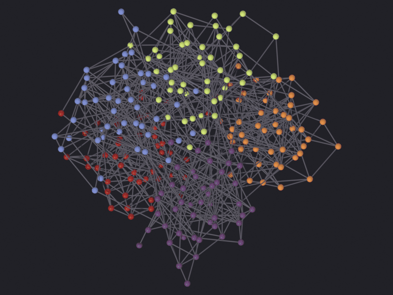
A layout therefore asserts that these nodes belong near each other. Two nodes drawn close together in a force layout are claimed to be close in the graph; in a sphere layout they are claimed nothing, because that layout never looked at an edge. The picture does not distinguish the two, so every figure here says which algorithm made it.

Getting graphs into Blender is notebook 01; centrality is 17, algorithms 18, topology 19. No internet needed: the graph is generated.

0 · Setup

import pathlib
import sys


def find_repo():
    """Locate the SciGraphs repository, without relying on the cwd.

    In a normal Jupyter the kernel starts per notebook with the cwd set to its
    folder. Not here: the kernel lives inside Blender and existed before you
    opened anything, so the cwd is wherever Blender was launched from. What the
    extension does know is which folder it is serving to JupyterLab.
    """
    candidates = []
    try:
        import bpy
        prefs = bpy.context.preferences.addons[
            "bl_ext.user_default.jupyter_blender"].preferences
        candidates.append(pathlib.Path(bpy.path.abspath(prefs.notebook_dir)))
    except Exception:
        pass
    candidates.append(pathlib.Path.cwd())

    for base in candidates:
        for directory in (base, *base.parents):
            if (directory / "SciGraphs" / "api" / "graphs.py").is_file():
                return directory

    raise RuntimeError(
        "Cannot find the SciGraphs repository. Point at it by hand:\n"
        "    sys.path.insert(0, '/path/to/SciGraphs-1/notebooks/tools')")


sys.path.insert(0, str(find_repo() / "notebooks" / "tools"))

import time

import bpy
import networkx as nx
import numpy as np

# `nb` must import first: it puts this repository on sys.path, so the
# `SciGraphs` import below reads this tree, not the copy Blender installed.
import nb
from nb import check

from SciGraphs import api as sg

from scigraphs_core.algorithms.graph import GraphData
from SciGraphs.core.mesh import geometry
from scigraphs_core.mesh import layout as sglayout
from scigraphs_core.mesh.layouts.common import _build_networkx_graph
from scigraphs_core.mesh.layouts.yifan_hu import _has_isolated_node
from scigraphs_core.repro import determinism

print("networkx", nx.__version__)

scigraphs-utils available - Graphviz layouts enabled
networkx 3.6

1 · A graph with no positions

The structure has to be known, or there is no way to say whether a layout found it or invented it. A stochastic block model gives that: five groups of forty-eight nodes, dense inside a group and sparse between them, the group recorded per node, nothing about position. The seed is fixed, because a claim about reproducibility is worth nothing measured on a graph that was itself different each time.

BLOCKS = 5
PER_BLOCK = 48
P_IN, P_OUT = 0.12, 0.006
GRAPH_SEED = 11

probabilities = [[P_IN if i == j else P_OUT for j in range(BLOCKS)]
                 for i in range(BLOCKS)]
G = nx.stochastic_block_model([PER_BLOCK] * BLOCKS, probabilities,
                              seed=GRAPH_SEED)

# Both steps are load-bearing: an isolated node aborts one of the layout
# backends outright (section 8), and the mesh builder indexes nodes by
# position.
G = G.subgraph(max(nx.connected_components(G), key=len)).copy()
G = nx.convert_node_labels_to_integers(G, ordering="sorted",
                                       label_attribute="original")

block = np.array([G.nodes[n]["block"] for n in G.nodes()], dtype=np.int32)
degree = np.array([d for _, d in sorted(G.degree())], dtype=np.float32)

print(f"nodes {G.number_of_nodes()}, edges {G.number_of_edges()}")
print(f"blocks {BLOCKS} x {PER_BLOCK}, kept {np.bincount(block).tolist()}")
print(f"degree: min {degree.min():.0f}  median {np.median(degree):.0f}  "
      f"max {degree.max():.0f}")

inside = sum(1 for u, v in G.edges() if block[u] == block[v])
print(f"edges inside a block: {inside} of {G.number_of_edges()} "
      f"({inside / G.number_of_edges() * 100:.0f}%)")

check("the graph is connected", nx.is_connected(G))
check("no isolated node", min(dict(G.degree()).values()) > 0,
      "section 8 explains why this is checked here")

nodes 240, edges 840
blocks 5 x 48, kept [48, 48, 48, 48, 48]
degree: min 1  median 7  max 14
edges inside a block: 690 of 840 (82%)
[PASS] the graph is connected
[PASS] no isolated node — section 8 explains why this is checked here

True

Into Blender

create_graph_object is the mesh builder for a non-geospatial graph: one vertex per node, one mesh edge per pair, node and edge lists stored as strings on the object (notebook 01 covers the import routes that call it). Two things bite headlessly. It links the new object through bpy.context.collection, which is None under blender -b in some scenes (the trap notebook 11 hit), so an explicit collection inside a temp_override is used instead. And the initial positions are random, from repro.determinism.get_geometry_seed(): every figure before the first apply_layout is a picture of a random number generator.

sg.graphs.clear_scene(keep_anchor=False)
COLL = sg.graphs.collection("SG_Layouts")

print("geometry seed:", determinism.get_geometry_seed())
print("layout seed  :", determinism.get_layout_seed())

with nb.quiet():
    with bpy.context.temp_override(collection=COLL):
        graph = geometry.create_graph_object(GraphData(list(G.nodes()),
                                             list(G.edges())))
graph.name = "SBM_240"
sg.graphs.activate(graph)

print(sg.graphs.summary(graph))

geometry seed: 1426602425
layout seed  : 981798123

Creating graph object with 240 nodes...
  Random positions generated in 0.00s (seed=1426602425)
  Vertices created in 0.00s
  840 edges created in 0.00s
  Mesh conversion in 0.00s
  Object created in 0.00s
Total graph creation time: 0.00s
{'object': 'SBM_240', 'type': 'MESH', 'num_nodes': 240, 'num_edges': 840, 'is_directed': False, 'vertices': 240, 'mesh_edges': 840, 'attributes': ['position', '.edge_verts', '.corner_vert', '.corner_edge']}

What the layout receives is not the mesh. apply_graph_layout rebuilds a NetworkX graph from the object’s nodes_data and edges_data, falling back to the mesh edges only when edges_data is empty. A mesh with four thousand edges whose edges_data is blank reaches the layout as four hundred isolated points: a wrong picture and, for one backend, a crash. Check it on any object of uncertain provenance.

seen, seen_n = _build_networkx_graph(graph)
isolated = sum(1 for _, d in seen.degree() if d == 0)
print(f"the layout sees {seen.number_of_nodes()} nodes, "
      f"{seen.number_of_edges()} edges, {isolated} isolated")

check("the layout sees the same graph the mesh does",
      seen.number_of_nodes() == G.number_of_nodes()
      and seen.number_of_edges() == G.number_of_edges(),
      f"{seen.number_of_edges()} vs {G.number_of_edges()} edges")

the layout sees 240 nodes, 840 edges, 0 isolated
[PASS] the layout sees the same graph the mesh does — 840 vs 840 edges

True

The two attributes every figure here is colored by

node_block is the group each node was generated in: ground truth, known before any layout ran, identical in every panel. When the only thing that changes between two figures is the algorithm, a color that does not change is the only way to see they are the same graph. node_degree is for the sections asking about a node rather than a group.

def put_attribute(obj, name, values, domain='POINT'):
    """Write (or overwrite) a float attribute on the mesh."""
    values = np.asarray(values, dtype=np.float32).ravel()
    existing = obj.data.attributes.get(name)
    if existing is not None:
        obj.data.attributes.remove(existing)
    attribute = obj.data.attributes.new(name, 'FLOAT', domain)
    attribute.data.foreach_set("value", values)
    obj.data.update()
    return name


put_attribute(graph, "node_block", block)
put_attribute(graph, "node_degree", degree)

for name, domain, dtype in sg.graphs.attributes(graph):
    if not name.startswith("."):
        print(f"  {name:<16} {domain:<7} {dtype}")

  position         POINT   FLOAT_VECTOR
  node_block       POINT   FLOAT
  node_degree      POINT   FLOAT

Both attributes are on the nodes, and that is forced

Applying a layout zeroes every EDGE-domain attribute on the mesh. The layer survives, with the right name, domain and length; every value becomes 0. Nothing raises, and a figure colored by that attribute comes back a flat single color that looks like a colormap problem.

The cause is rebuild_edges, called by every layout operator after moving the nodes. It deletes every bmesh edge and creates them again from edges_data (SciGraphs/core/mesh/geometry.py:1227 to :1248), and a new edge has no custom data: the layer is re-allocated to the new edge count and filled with the default. Called from layout_operators.py:322 (Apply Layout), :397 (step-by-step), :483 (Reset), :589 and :639 (the 3D splitter), and from data_operators.py:41, the auto-layout that runs on import. A graph imported with auto-layout on has lost its edge columns before you have looked at it once.

# The layout below overwrites these, and the next figure is about them.
arrival = np.array(graph["node_positions"], dtype=np.float64)

edge_count = len(graph.data.edges)
put_attribute(graph, "edge_marker",
              np.arange(1, edge_count + 1, dtype=np.float32), domain='EDGE')
put_attribute(graph, "node_marker",
              np.arange(1, graph["num_nodes"] + 1, dtype=np.float32))


def read_attribute(obj, name, length):
    attribute = obj.data.attributes.get(name)
    if attribute is None:
        return None
    buffer = np.empty(length, dtype=np.float32)
    attribute.data.foreach_get("value", buffer)
    return buffer


before_edges = read_attribute(graph, "edge_marker", edge_count)
before_nodes = read_attribute(graph, "node_marker", graph["num_nodes"])
print(f"before: edge_marker sums to {before_edges.sum():.0f}, "
      f"node_marker to {before_nodes.sum():.0f}")

sg.graphs.activate(graph)
with nb.quiet():
    bpy.ops.scigraphs.apply_layout(algorithm='IGRAPH_KK', iterations=50,
                                   scale=5.0)

after_edges = read_attribute(graph, "edge_marker", len(graph.data.edges))
after_nodes = read_attribute(graph, "node_marker", graph["num_nodes"])
print(f"after : edge_marker sums to {after_edges.sum():.0f}, "
      f"node_marker to {after_nodes.sum():.0f}")
print(f"        the edge layer is still there: "
      f"{sg.render.attribute_domain(graph, 'edge_marker')}, "
      f"{len(graph.data.edges)} values, all "
      f"{after_edges.min():.0f}")

check("a layout preserves node attributes",
      np.array_equal(before_nodes, after_nodes))
check("a layout destroys edge attributes",
      float(np.abs(after_edges).max()) == 0.0,
      "the layer survives with every value set to zero, silently")

before: edge_marker sums to 353220, node_marker to 28920
Computing igraph Kamada-Kawai layout for 240 nodes...
  Kamada-Kawai completed in 0.05s

======================================================================
Layout algorithm: IGRAPH_KK
Graph: 240 nodes, 840 edges
Parameters:
  - algorithm: IGRAPH_KK
  - iterations: 50
  - scale: 5.0000
  - num_nodes: 240
  - num_edges: 840
Execution time: 0.056s
Status: success
======================================================================

Info: Layout 'IGRAPH_KK' applied
after : edge_marker sums to 0, node_marker to 28920
        the edge layer is still there: EDGE, 840 values, all 0
[PASS] a layout preserves node attributes
[PASS] a layout destroys edge attributes — the layer survives with every value set to zero, silently

True

The order of operations is therefore load-bearing:

1. import the graph, with auto-layout off;
2. lay it out;
3. then compute or import anything edge-valued, and color by it.

Anything edge-valued computed before step 2 has to be recomputed after it. Node attributes are unaffected (node_marker came through untouched), which is why this notebook’s colors are all on the nodes and section 4 can re-run seven layouts on one object.

for name in ("edge_marker", "node_marker"):
    graph.data.attributes.remove(graph.data.attributes[name])

graph["node_positions"] = arrival.flatten().tolist()
geometry.update_node_positions_from_property(graph)
geometry.rebuild_edges(graph)
check("the arrival positions are back",
      float(np.abs(np.array(graph["node_positions"],
      dtype=np.float64) - arrival).max()) < 1e-9)

[PASS] the arrival positions are back

True

What you are looking at, and why it is that color. Every figure here is taken straight down through an orthographic camera (render_eevee’s default) with look='ink', the house style from notebook 13 onwards: a near-black backdrop and turbo, whose low end is a dark blue rather than the black that would swallow it. Turbo is read by hue, not brightness; notebook 16 measures what that costs. Five categories rather than a continuum is the one job where the ramp’s uneven spacing does no harm.

Node size is re-derived on every render, which matters more here than anywhere else in the suite: the same 240 nodes span 5.4 Blender units under one algorithm and 140 under another (section 4), so a radius that reads under one is a mat under the next. render_eevee sizes each glyph at 0.35 of the median nearest-neighbor distance of the positions it is about to draw, and the radii are printed with the panels.

One guard before the first figure

Seven layouts go through one camera and their extents differ by a factor of twenty-six, so a framing that depends on anything but the graph in front of it, such as a camera left at the previous panel’s scale, would show here first. Frame the same graph four times from a camera reset to Blender’s default and see whether the four agree.

sg.render.autoscale_geometry(graph, verbose=False)
bpy.context.scene.render.resolution_x = 1000
bpy.context.scene.render.resolution_y = 750

sg.render.frame_camera(graph).data.ortho_scale = 6.0
fits = [sg.render.frame_camera(graph).data.ortho_scale for _ in range(4)]
print("ortho_scale over four identical framing calls, from a default camera:")
print("  " + "  ".join(f"{value:.3f}" for value in fits))

check("the framing depends on the graph and on nothing else",
      max(fits) - min(fits) < 1e-6,
      "it did not always: this call used to be solved iteratively "
      "against the camera's current state, and the first framing of a "
      "session came out short enough to cut the outermost nodes in half")

ortho_scale over four identical framing calls, from a default camera:
  7.506  7.506  7.506  7.506
[PASS] the framing depends on the graph and on nothing else — it did not always: this call used to be solved iteratively against the camera's current state, and the first framing of a session came out short enough to cut the outermost nodes in half

True

Necessary, not sufficient: a repeatable frame can still be the wrong size. Every figure below goes through a wrapper that frames the camera, measures whether the graph and one node radius around every node is inside the frame, and raises the margin until it is, saying so when it has to.

def framing_margin(obj, resolution, margin=sg.render.FRAME_MARGIN):
    """The smallest margin that actually contains the graph. Measured."""
    scene = bpy.context.scene
    scene.render.resolution_x, scene.render.resolution_y = resolution
    sg.render.autoscale_geometry(obj, verbose=False)
    radius = float(obj.get("scigraphs_node_size", 0.0) or 0.0)

    for _ in range(6):
        cam = sg.render.frame_camera(obj, margin=margin)
        width, height = sg.render._frame_extent(cam)
        points = sg.render._fit_points(obj, radius)
        lo, hi = points.min(axis=0), points.max(axis=0)
        need = max(2.0 * max(cam.location.x - lo[0], hi[0] - cam.location.x) / width,
                   2.0 * max(cam.location.y - lo[1], hi[1] - cam.location.y) / height)
        if need <= 1.0:
            return margin
        margin *= need * 1.01
    return margin


def draw(obj, filename, resolution=(1000, 750), width=900, **kwargs):
    """`draw_eevee`, with the framing checked instead of assumed."""
    margin = framing_margin(obj, resolution)
    if margin > sg.render.FRAME_MARGIN * 1.001:
        print(f"  framing margin raised {sg.render.FRAME_MARGIN:.2f} -> "
              f"{margin:.2f}; the fitted frame would have cropped the graph")
    return nb.figure(obj, filename, resolution=resolution,
                     width=width, margin=margin, **kwargs)

draw(graph, "renders/14_layouts/1_as_it_arrives",
     look='ink', color_attribute="node_block")

Info: Geometry Nodes modifier added
Info: Attribute -> node_block  ·  node_block -> turbo [log]  [0 … 4] on Point

[PASS] 1_as_it_arrives.png legible — 55.2% ink (healthy range 0.5–60%)

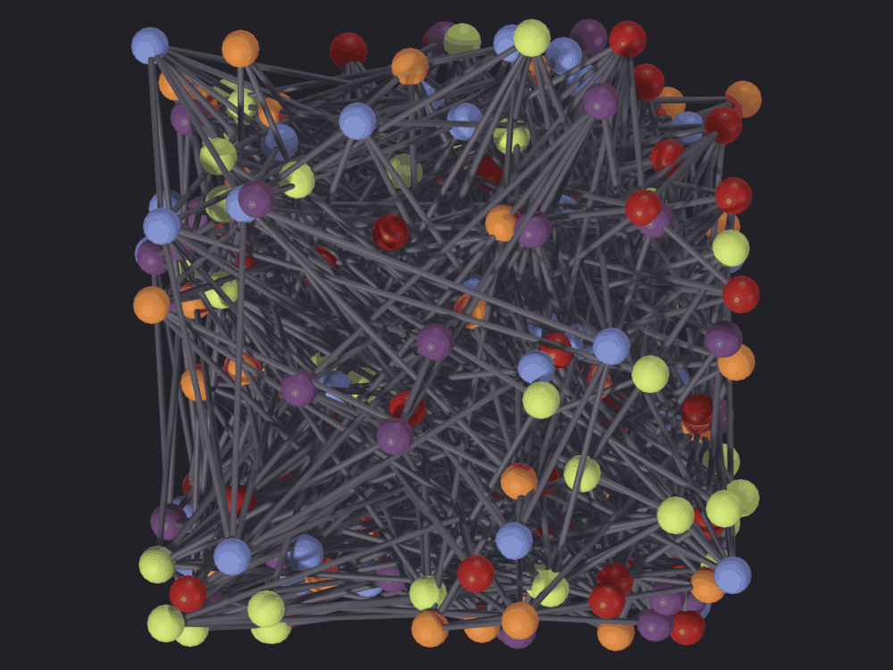
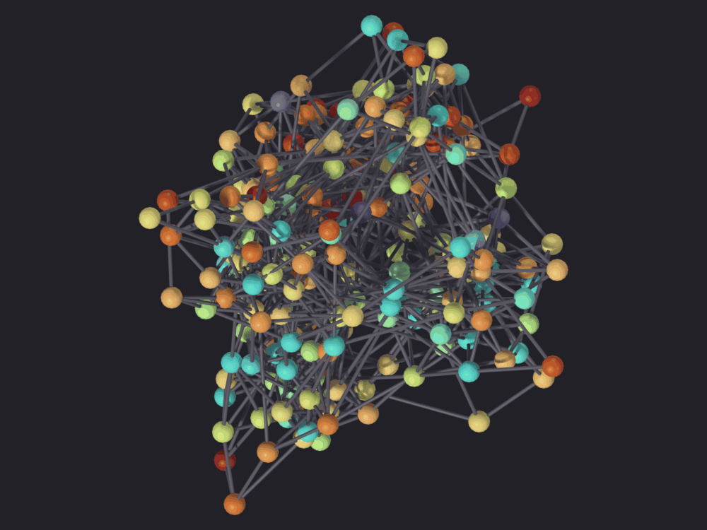
The graph as the mesh builder left it: 240 nodes at random positions in a cube, 840 edges between them, every group spread across the whole frame. The control the rest of the notebook is measured against.

2 · The menu behind one enum

bpy.ops.scigraphs.apply_layout(algorithm=...) accepts thirty-two values. They belong to five families that answer different questions, and three of the entries are not layouts of the graph at all.

FAMILIES = {
    "force-directed": ['SPRING', 'SPRING_3D', 'FORCEATLAS2', 'IGRAPH_FR',
                       'IGRAPH_DRL', 'IGRAPH_DRL_2D', 'IGRAPH_LGL',
                       'IGRAPH_DH', 'IGRAPH_GRAPHOPT', 'YIFAN_HU',
                       'GRAPHVIZ_NEATO', 'GRAPHVIZ_FDP', 'GRAPHVIZ_SFDP'],
    "stress / spectral": ['IGRAPH_KK', 'SPECTRAL_3D', 'MDS_3D'],
    "hierarchical": ['GRAPHVIZ_DOT', 'SUGIYAMA', 'HIERARCHICAL_3D',
                     'CIRCULAR_HIERARCHY', 'BIPARTITE_3D', 'GRAPHVIZ_TWOPI'],
    "circular / packing": ['GRAPHVIZ_CIRCO', 'CIRCLE_PACKING',
                           'GRAPHVIZ_OSAGE', 'GRAPHVIZ_PATCHWORK'],
    "geometric (ignores the edges)": ['RANDOM', 'GRID', 'SPHERE', 'SPIRAL_3D',
                                      'HELIX', 'CUBE'],
}

listed = {item for group in FAMILIES.values() for item in group}
enum = {item.identifier for item in
        bpy.ops.scigraphs.apply_layout.get_rna_type()
        .properties["algorithm"].enum_items}

print(f"{'family':<32} {'n':>3}  what it is optimizing")
print("-" * 78)
for family, members in FAMILIES.items():
    print(f"{family:<32} {len(members):>3}")
print()
print("in the enum but unclassified:", sorted(enum - listed) or "none")
print("classified but not in the enum:", sorted(listed - enum) or "none")

check("every algorithm in the enum is accounted for",
      listed == enum, f"{len(enum)} entries")

family                             n  what it is optimizing
------------------------------------------------------------------------------
force-directed                    13
stress / spectral                  3
hierarchical                       6
circular / packing                 4
geometric (ignores the edges)      6

in the enum but unclassified: none
classified but not in the enum: none
[PASS] every algorithm in the enum is accounted for — 32 entries

True

The last family is the one to be careful with. SPHERE, HELIX, SPIRAL_3D, GRID and RANDOM never read an edge: they place node i by i and the node count. They are legitimate (a sphere of nodes with edges drawn between them shows that a graph is dense) but a figure made with one cannot support a claim about structure, and section 4 shows one of them scoring well for a reason that has nothing to do with the graph.

What is actually installed

Several branches are optional and fall back silently. The operator reports FINISHED either way and the only trace is a console line.

from scigraphs_core.mesh.layouts import common as layout_common
from scigraphs_core.mesh.layouts import forceatlas as layout_fa2

print(f"igraph available          : {layout_common.IGRAPH_AVAILABLE}")
print(f"scigraphs-utils (Graphviz): {layout_common.GRAPHVIZ_AVAILABLE}")
print(f"fa2 package               : {layout_common.FA2_AVAILABLE}")
print(f"networkx forceatlas2      : {layout_fa2.NX_FA2 is not None}")

check("igraph is present", layout_common.IGRAPH_AVAILABLE,
      "without it, nine algorithms silently become Spring 2D")
check("the Graphviz backend is present", layout_common.GRAPHVIZ_AVAILABLE,
      "without it, YIFAN_HU and the eight GRAPHVIZ_* entries fail")

igraph available          : True
scigraphs-utils (Graphviz): True
fa2 package               : False
networkx forceatlas2      : True
[PASS] igraph is present — without it, nine algorithms silently become Spring 2D
[PASS] the Graphviz backend is present — without it, YIFAN_HU and the eight GRAPHVIZ_* entries fail

True

Add-on defect: a fallback that is announced but does not happen. FORCEATLAS2 is the scene default (layout_algorithm), and the optional fa2 package is not installed in Blender’s Python. The dispatcher treats that as a fallback and labels the run so (SciGraphs/core/mesh/layouts/dispatcher.py:58), printing

Computing ForceAtlas2 (3D, networkx) for 240 nodes...
Layout algorithm: FORCEATLAS2
Fallback: using SPRING (2D fallback) instead
   Reason: FORCEATLAS2 library not available

The first line is the true one: what ran was ForceAtlas2, in 3D. _forceatlas2_layout prefers nx.forceatlas2_layout, which networkx has had since 3.4 (SciGraphs/core/mesh/layouts/forceatlas.py:24), and drops to Spring 2D only when neither backend exists. The label is checked against FA2_AVAILABLE alone, never against what the function chose. The same test guards the nine IGRAPH_* branches, where it is correct because those do fall through.

The object cannot be asked either: the import path stamps obj["auto_layout_algorithm"] = props.layout_algorithm (SciGraphs/ui/operators/scigraphs/data_operators.py:42), the algorithm requested. A graph laid out by a fallback carries the name of the algorithm that was not available.

3 · Is a layout a function of the graph?

Before comparing seven layouts, is one layout a stable thing? A force layout starts from random positions, and the machinery is there: apply_graph_layout opens by calling _reset_layout_rng(), which seeds a module-level RandomState from repro.determinism.get_layout_seed().

Each algorithm runs three times rather than twice, because one of the results below is that the first run differs from every later one.

def positions(obj):
    """The layout's node positions as an (n, 3) array. A **copy**.

    `np.asarray` would not do. A Blender ID property array supports the buffer
    protocol, so `asarray` hands back a *view* onto Blender's own memory, and
    Blender reuses that allocation when the property is overwritten with a list
    of the same length. Two "before and after" snapshots taken that way are the
    same object, every difference between them is exactly zero, and nothing
    raises.
    """
    return np.array(obj["node_positions"], dtype=np.float64).reshape(-1, 3)


def apply(obj, algorithm, iterations=100, scale=5.0, **kwargs):
    """`bpy.ops.scigraphs.apply_layout`, timed, quiet, returning positions."""
    sg.graphs.activate(obj)
    started = time.time()
    with nb.quiet():
        result = bpy.ops.scigraphs.apply_layout(
            algorithm=algorithm, iterations=iterations, scale=scale, **kwargs)
    elapsed = time.time() - started
    if 'FINISHED' not in result:
        return None, elapsed
    return positions(obj), elapsed


# YIFAN_HU before GRAPHVIZ_SFDP: same Graphviz engine, and only whichever runs
# first in the process sees what section 3.1 describes.
REPEATED = ['GRID', 'RANDOM', 'SPHERE', 'CUBE', 'FORCEATLAS2', 'SPRING_3D',
            'IGRAPH_FR', 'IGRAPH_KK', 'SPECTRAL_3D', 'MDS_3D', 'YIFAN_HU',
            'GRAPHVIZ_SFDP', 'GRAPHVIZ_DOT']

repeats = {}
for algorithm in REPEATED:
    runs = []
    for _ in range(3):
        pos, _elapsed = apply(graph, algorithm)
        runs.append(pos)
    if any(r is None for r in runs):
        repeats[algorithm] = None
        continue
    repeats[algorithm] = {
        "xy_1v2": float(np.abs(runs[0][:, :2] - runs[1][:, :2]).max()),
        "xy_2v3": float(np.abs(runs[1][:, :2] - runs[2][:, :2]).max()),
        "z_1v2": float(np.abs(runs[0][:, 2] - runs[1][:, 2]).max()),
        "z_2v3": float(np.abs(runs[1][:, 2] - runs[2][:, 2]).max()),
        "extent": float(np.linalg.norm(runs[2].max(axis=0) - runs[2].min(axis=0))),
    }

print(f"{'algorithm':<16}{'extent':>9}{'xy 1v2':>10}{'xy 2v3':>10}"
      f"{'z 1v2':>9}{'z 2v3':>9}   verdict")
print("-" * 78)
for algorithm, r in repeats.items():
    if r is None:
        print(f"{algorithm:<16}{'-':>9}   did not finish")
        continue
    worst_later = max(r["xy_2v3"], r["z_2v3"])
    worst_first = max(r["xy_1v2"], r["z_1v2"])
    if worst_first <= 1e-9:
        verdict = "repeats"
    elif worst_later <= 1e-9:
        verdict = "repeats from the 2nd run on"
    else:
        verdict = "does not repeat"
    print(f"{algorithm:<16}{r['extent']:9.2f}{r['xy_1v2']:10.4f}"
          f"{r['xy_2v3']:10.4f}{r['z_1v2']:9.4f}{r['z_2v3']:9.4f}   {verdict}")

======================================================================
Layout algorithm: GRID
Graph: 240 nodes, 840 edges
Parameters:
  - algorithm: GRID
  - iterations: 100
  - scale: 5.0000
  - num_nodes: 240
  - num_edges: 840
Execution time: 0.001s
Status: success
======================================================================

Info: Layout 'GRID' applied

======================================================================
Layout algorithm: GRID
Graph: 240 nodes, 840 edges
Parameters:
  - algorithm: GRID
  - iterations: 100
  - scale: 5.0000
  - num_nodes: 240
  - num_edges: 840
Execution time: 0.001s
Status: success
======================================================================

Info: Layout 'GRID' applied

======================================================================
Layout algorithm: GRID
Graph: 240 nodes, 840 edges
Parameters:
  - algorithm: GRID
  - iterations: 100
  - scale: 5.0000
  - num_nodes: 240
  - num_edges: 840
Execution time: 0.001s
Status: success
======================================================================

Info: Layout 'GRID' applied

======================================================================
Layout algorithm: RANDOM
Graph: 240 nodes, 840 edges
Parameters:
  - algorithm: RANDOM
  - iterations: 100
  - scale: 5.0000
  - num_nodes: 240
  - num_edges: 840
Execution time: 0.001s
Status: success
======================================================================

Info: Layout 'RANDOM' applied

======================================================================
Layout algorithm: RANDOM
Graph: 240 nodes, 840 edges
Parameters:
  - algorithm: RANDOM
  - iterations: 100
  - scale: 5.0000
  - num_nodes: 240
  - num_edges: 840
Execution time: 0.001s
Status: success
======================================================================

Info: Layout 'RANDOM' applied

======================================================================
Layout algorithm: RANDOM
Graph: 240 nodes, 840 edges
Parameters:
  - algorithm: RANDOM
  - iterations: 100
  - scale: 5.0000
  - num_nodes: 240
  - num_edges: 840
Execution time: 0.001s
Status: success
======================================================================

Info: Layout 'RANDOM' applied

======================================================================
Layout algorithm: SPHERE
Graph: 240 nodes, 840 edges
Parameters:
  - algorithm: SPHERE
  - iterations: 100
  - scale: 5.0000
  - num_nodes: 240
  - num_edges: 840
Execution time: 0.001s
Status: success
======================================================================

Info: Layout 'SPHERE' applied

======================================================================
Layout algorithm: SPHERE
Graph: 240 nodes, 840 edges
Parameters:
  - algorithm: SPHERE
  - iterations: 100
  - scale: 5.0000
  - num_nodes: 240
  - num_edges: 840
Execution time: 0.001s
Status: success
======================================================================

Info: Layout 'SPHERE' applied

======================================================================
Layout algorithm: SPHERE
Graph: 240 nodes, 840 edges
Parameters:
  - algorithm: SPHERE
  - iterations: 100
  - scale: 5.0000
  - num_nodes: 240
  - num_edges: 840
Execution time: 0.001s
Status: success
======================================================================

Info: Layout 'SPHERE' applied

======================================================================
Layout algorithm: CUBE
Graph: 240 nodes, 840 edges
Parameters:
  - algorithm: CUBE
  - iterations: 100
  - scale: 5.0000
  - num_nodes: 240
  - num_edges: 840
Execution time: 0.001s
Status: success
======================================================================

Info: Layout 'CUBE' applied

======================================================================
Layout algorithm: CUBE
Graph: 240 nodes, 840 edges
Parameters:
  - algorithm: CUBE
  - iterations: 100
  - scale: 5.0000
  - num_nodes: 240
  - num_edges: 840
Execution time: 0.001s
Status: success
======================================================================

Info: Layout 'CUBE' applied

======================================================================
Layout algorithm: CUBE
Graph: 240 nodes, 840 edges
Parameters:
  - algorithm: CUBE
  - iterations: 100
  - scale: 5.0000
  - num_nodes: 240
  - num_edges: 840
Execution time: 0.002s
Status: success
======================================================================

Info: Layout 'CUBE' applied
Computing ForceAtlas2 (3D, networkx) for 240 nodes...
  ForceAtlas2 completed in 0.18s

======================================================================
Layout algorithm: FORCEATLAS2
Fallback: using SPRING (2D fallback) instead
   Reason: FORCEATLAS2 library not available
Graph: 240 nodes, 840 edges
Parameters:
  - algorithm: FORCEATLAS2
  - iterations: 100
  - scale: 5.0000
  - num_nodes: 240
  - num_edges: 840
Execution time: 0.178s
Status: success (with fallback)
======================================================================

Info: Layout 'FORCEATLAS2' applied
Computing ForceAtlas2 (3D, networkx) for 240 nodes...
  ForceAtlas2 completed in 0.18s

======================================================================
Layout algorithm: FORCEATLAS2
Fallback: using SPRING (2D fallback) instead
   Reason: FORCEATLAS2 library not available
Graph: 240 nodes, 840 edges
Parameters:
  - algorithm: FORCEATLAS2
  - iterations: 100
  - scale: 5.0000
  - num_nodes: 240
  - num_edges: 840
Execution time: 0.180s
Status: success (with fallback)
======================================================================

Info: Layout 'FORCEATLAS2' applied
Computing ForceAtlas2 (3D, networkx) for 240 nodes...
  ForceAtlas2 completed in 0.18s

======================================================================
Layout algorithm: FORCEATLAS2
Fallback: using SPRING (2D fallback) instead
   Reason: FORCEATLAS2 library not available
Graph: 240 nodes, 840 edges
Parameters:
  - algorithm: FORCEATLAS2
  - iterations: 100
  - scale: 5.0000
  - num_nodes: 240
  - num_edges: 840
Execution time: 0.178s
Status: success (with fallback)
======================================================================

Info: Layout 'FORCEATLAS2' applied

======================================================================
Layout algorithm: SPRING_3D
Graph: 240 nodes, 840 edges
Parameters:
  - algorithm: SPRING_3D
  - iterations: 100
  - scale: 5.0000
  - num_nodes: 240
  - num_edges: 840
Execution time: 0.138s
Status: success
======================================================================

Info: Layout 'SPRING_3D' applied

======================================================================
Layout algorithm: SPRING_3D
Graph: 240 nodes, 840 edges
Parameters:
  - algorithm: SPRING_3D
  - iterations: 100
  - scale: 5.0000
  - num_nodes: 240
  - num_edges: 840
Execution time: 0.144s
Status: success
======================================================================

Info: Layout 'SPRING_3D' applied

======================================================================
Layout algorithm: SPRING_3D
Graph: 240 nodes, 840 edges
Parameters:
  - algorithm: SPRING_3D
  - iterations: 100
  - scale: 5.0000
  - num_nodes: 240
  - num_edges: 840
Execution time: 0.146s
Status: success
======================================================================

Info: Layout 'SPRING_3D' applied
Computing igraph Fruchterman-Reingold layout for 240 nodes...
  Fruchterman-Reingold completed in 0.01s

======================================================================
Layout algorithm: IGRAPH_FR
Graph: 240 nodes, 840 edges
Parameters:
  - algorithm: IGRAPH_FR
  - iterations: 100
  - scale: 5.0000
  - num_nodes: 240
  - num_edges: 840
Execution time: 0.012s
Status: success
======================================================================

Info: Layout 'IGRAPH_FR' applied
Computing igraph Fruchterman-Reingold layout for 240 nodes...
  Fruchterman-Reingold completed in 0.01s

======================================================================
Layout algorithm: IGRAPH_FR
Graph: 240 nodes, 840 edges
Parameters:
  - algorithm: IGRAPH_FR
  - iterations: 100
  - scale: 5.0000
  - num_nodes: 240
  - num_edges: 840
Execution time: 0.013s
Status: success
======================================================================

Info: Layout 'IGRAPH_FR' applied
Computing igraph Fruchterman-Reingold layout for 240 nodes...
  Fruchterman-Reingold completed in 0.01s

======================================================================
Layout algorithm: IGRAPH_FR
Graph: 240 nodes, 840 edges
Parameters:
  - algorithm: IGRAPH_FR
  - iterations: 100
  - scale: 5.0000
  - num_nodes: 240
  - num_edges: 840
Execution time: 0.013s
Status: success
======================================================================

Info: Layout 'IGRAPH_FR' applied
Computing igraph Kamada-Kawai layout for 240 nodes...
  Kamada-Kawai completed in 0.05s

======================================================================
Layout algorithm: IGRAPH_KK
Graph: 240 nodes, 840 edges
Parameters:
  - algorithm: IGRAPH_KK
  - iterations: 100
  - scale: 5.0000
  - num_nodes: 240
  - num_edges: 840
Execution time: 0.055s
Status: success
======================================================================

Info: Layout 'IGRAPH_KK' applied
Computing igraph Kamada-Kawai layout for 240 nodes...
  Kamada-Kawai completed in 0.05s

======================================================================
Layout algorithm: IGRAPH_KK
Graph: 240 nodes, 840 edges
Parameters:
  - algorithm: IGRAPH_KK
  - iterations: 100
  - scale: 5.0000
  - num_nodes: 240
  - num_edges: 840
Execution time: 0.055s
Status: success
======================================================================

Info: Layout 'IGRAPH_KK' applied
Computing igraph Kamada-Kawai layout for 240 nodes...
  Kamada-Kawai completed in 0.06s

======================================================================
Layout algorithm: IGRAPH_KK
Graph: 240 nodes, 840 edges
Parameters:
  - algorithm: IGRAPH_KK
  - iterations: 100
  - scale: 5.0000
  - num_nodes: 240
  - num_edges: 840
Execution time: 0.061s
Status: success
======================================================================

Info: Layout 'IGRAPH_KK' applied
Computing Spectral 3D layout for 240 nodes...
  Spectral 3D completed in 0.04s

======================================================================
Layout algorithm: SPECTRAL_3D
Graph: 240 nodes, 840 edges
Parameters:
  - algorithm: SPECTRAL_3D
  - iterations: 100
  - scale: 5.0000
  - num_nodes: 240
  - num_edges: 840
Execution time: 0.037s
Status: success
======================================================================

Info: Layout 'SPECTRAL_3D' applied
Computing Spectral 3D layout for 240 nodes...
  Spectral 3D completed in 0.03s

======================================================================
Layout algorithm: SPECTRAL_3D
Graph: 240 nodes, 840 edges
Parameters:
  - algorithm: SPECTRAL_3D
  - iterations: 100
  - scale: 5.0000
  - num_nodes: 240
  - num_edges: 840
Execution time: 0.036s
Status: success
======================================================================

Info: Layout 'SPECTRAL_3D' applied
Computing Spectral 3D layout for 240 nodes...
  Spectral 3D completed in 0.04s

======================================================================
Layout algorithm: SPECTRAL_3D
Graph: 240 nodes, 840 edges
Parameters:
  - algorithm: SPECTRAL_3D
  - iterations: 100
  - scale: 5.0000
  - num_nodes: 240
  - num_edges: 840
Execution time: 0.036s
Status: success
======================================================================

Info: Layout 'SPECTRAL_3D' applied
Computing MDS 3D layout for 240 nodes...
  MDS 3D completed in 0.11s

======================================================================
Layout algorithm: MDS_3D
Graph: 240 nodes, 840 edges
Parameters:
  - algorithm: MDS_3D
  - iterations: 100
  - scale: 5.0000
  - num_nodes: 240
  - num_edges: 840
Execution time: 0.111s
Status: success
======================================================================

Info: Layout 'MDS_3D' applied
Computing MDS 3D layout for 240 nodes...
  MDS 3D completed in 0.07s

======================================================================
Layout algorithm: MDS_3D
Graph: 240 nodes, 840 edges
Parameters:
  - algorithm: MDS_3D
  - iterations: 100
  - scale: 5.0000
  - num_nodes: 240
  - num_edges: 840
Execution time: 0.067s
Status: success
======================================================================

Info: Layout 'MDS_3D' applied
Computing MDS 3D layout for 240 nodes...
  MDS 3D completed in 0.06s

======================================================================
Layout algorithm: MDS_3D
Graph: 240 nodes, 840 edges
Parameters:
  - algorithm: MDS_3D
  - iterations: 100
  - scale: 5.0000
  - num_nodes: 240
  - num_edges: 840
Execution time: 0.059s
Status: success
======================================================================

Info: Layout 'MDS_3D' applied
Computing Yifan Hu layout for 240 nodes...
  mode=2Z, backend=scigraphs-utils, engine=sfdp
  z_method=SPECTRAL, z_scale=0.30000001192092896
  Generated Graphviz Z via SPECTRAL: -0.750 to 0.212
  scigraphs-utils Graphviz sfdp computed 240 nodes
  Z range: -0.750 to 0.212
  Final ranges (scale=5.0): X=5.0, Y=4.5, Z=1.0
  Yifan Hu (scigraphs-utils sfdp, mode=2Z) completed in 0.05s

======================================================================
Layout algorithm: YIFAN_HU
Graph: 240 nodes, 840 edges
Parameters:
  - algorithm: YIFAN_HU
  - iterations: 100
  - scale: 5.0000
  - num_nodes: 240
  - num_edges: 840
Execution time: 0.055s
Status: success
======================================================================

Info: Layout 'YIFAN_HU' applied
Computing Yifan Hu layout for 240 nodes...
  mode=2Z, backend=scigraphs-utils, engine=sfdp
  z_method=SPECTRAL, z_scale=0.30000001192092896
  Generated Graphviz Z via SPECTRAL: -0.750 to 0.212
  scigraphs-utils Graphviz sfdp computed 240 nodes
  Z range: -0.750 to 0.212
  Final ranges (scale=5.0): X=5.0, Y=4.8, Z=1.0
  Yifan Hu (scigraphs-utils sfdp, mode=2Z) completed in 0.04s

======================================================================
Layout algorithm: YIFAN_HU
Graph: 240 nodes, 840 edges
Parameters:
  - algorithm: YIFAN_HU
  - iterations: 100
  - scale: 5.0000
  - num_nodes: 240
  - num_edges: 840
Execution time: 0.046s
Status: success
======================================================================

Info: Layout 'YIFAN_HU' applied
Computing Yifan Hu layout for 240 nodes...
  mode=2Z, backend=scigraphs-utils, engine=sfdp
  z_method=SPECTRAL, z_scale=0.30000001192092896
  Generated Graphviz Z via SPECTRAL: -0.212 to 0.750
  scigraphs-utils Graphviz sfdp computed 240 nodes
  Z range: -0.212 to 0.750
  Final ranges (scale=5.0): X=5.0, Y=4.8, Z=1.0
  Yifan Hu (scigraphs-utils sfdp, mode=2Z) completed in 0.04s

======================================================================
Layout algorithm: YIFAN_HU
Graph: 240 nodes, 840 edges
Parameters:
  - algorithm: YIFAN_HU
  - iterations: 100
  - scale: 5.0000
  - num_nodes: 240
  - num_edges: 840
Execution time: 0.041s
Status: success
======================================================================

Info: Layout 'YIFAN_HU' applied
  scigraphs-utils Graphviz sfdp computed 240 nodes

======================================================================
Layout algorithm: GRAPHVIZ_SFDP
Graph: 240 nodes, 840 edges
Parameters:
  - algorithm: GRAPHVIZ_SFDP
  - iterations: 100
  - scale: 5.0000
  - num_nodes: 240
  - num_edges: 840
Execution time: 0.034s
Status: success
======================================================================

Info: Layout 'GRAPHVIZ_SFDP' applied
  scigraphs-utils Graphviz sfdp computed 240 nodes

======================================================================
Layout algorithm: GRAPHVIZ_SFDP
Graph: 240 nodes, 840 edges
Parameters:
  - algorithm: GRAPHVIZ_SFDP
  - iterations: 100
  - scale: 5.0000
  - num_nodes: 240
  - num_edges: 840
Execution time: 0.035s
Status: success
======================================================================

Info: Layout 'GRAPHVIZ_SFDP' applied
  scigraphs-utils Graphviz sfdp computed 240 nodes

======================================================================
Layout algorithm: GRAPHVIZ_SFDP
Graph: 240 nodes, 840 edges
Parameters:
  - algorithm: GRAPHVIZ_SFDP
  - iterations: 100
  - scale: 5.0000
  - num_nodes: 240
  - num_edges: 840
Execution time: 0.035s
Status: success
======================================================================

Info: Layout 'GRAPHVIZ_SFDP' applied
  scigraphs-utils Graphviz dot computed 240 nodes

======================================================================
Layout algorithm: GRAPHVIZ_DOT
Graph: 240 nodes, 840 edges
Parameters:
  - algorithm: GRAPHVIZ_DOT
  - iterations: 100
  - scale: 5.0000
  - num_nodes: 240
  - num_edges: 840
Execution time: 0.440s
Status: success
======================================================================

Info: Layout 'GRAPHVIZ_DOT' applied
  scigraphs-utils Graphviz dot computed 240 nodes

======================================================================
Layout algorithm: GRAPHVIZ_DOT
Graph: 240 nodes, 840 edges
Parameters:
  - algorithm: GRAPHVIZ_DOT
  - iterations: 100
  - scale: 5.0000
  - num_nodes: 240
  - num_edges: 840
Execution time: 0.445s
Status: success
======================================================================

Info: Layout 'GRAPHVIZ_DOT' applied
  scigraphs-utils Graphviz dot computed 240 nodes

======================================================================
Layout algorithm: GRAPHVIZ_DOT
Graph: 240 nodes, 840 edges
Parameters:
  - algorithm: GRAPHVIZ_DOT
  - iterations: 100
  - scale: 5.0000
  - num_nodes: 240
  - num_edges: 840
Execution time: 0.435s
Status: success
======================================================================

Info: Layout 'GRAPHVIZ_DOT' applied
algorithm          extent    xy 1v2    xy 2v3    z 1v2    z 2v3   verdict
------------------------------------------------------------------------------
GRID                 6.41    0.0000    0.0000   0.0000   0.0000   repeats
RANDOM               8.59    0.0000    0.0000   0.0000   0.0000   repeats
SPHERE              17.27    0.0000    0.0000   0.0000   0.0000   repeats
CUBE                17.32    9.7057    9.6664   9.4661   9.4908   does not repeat
FORCEATLAS2         14.19    0.0000    0.0000   0.0000   0.0000   repeats
SPRING_3D           16.10    6.2090    8.8256   5.1653   6.0701   does not repeat
IGRAPH_FR          140.83   65.0302   60.4492  35.1703  75.9079   does not repeat
IGRAPH_KK          132.87    0.0000    0.0000   0.0000   0.0000   repeats
SPECTRAL_3D          7.52    0.0000    0.0000   0.0000   0.0000   repeats
MDS_3D              40.69    0.0000    0.0000   0.0000   0.0000   repeats
YIFAN_HU             6.99    5.0587    0.0000   0.0000   1.5000   does not repeat
GRAPHVIZ_SFDP        6.93    0.0000    0.0000   0.0000   0.0000   repeats
GRAPHVIZ_DOT         5.45    0.0000    0.0000   0.0000   0.0000   repeats

Three behaviors, only one of which the seeding machinery promises.

Deterministic. GRID, SPHERE, IGRAPH_KK, SPECTRAL_3D, MDS_3D, GRAPHVIZ_DOT and RANDOM return the same coordinates every time. The first six have no random component: Kamada-Kawai is stress majorization from a deterministic start, spectral and MDS are eigendecompositions, dot a layered sweep. RANDOM is random and reproducible: it draws from get_layout_seed() through _random_layout, a fixed function of the seed.

FORCEATLAS2 is the only force layout here that repeats, and the only one that consults the module RNG the dispatcher just reset: forceatlas.py:39 passes seed=_get_layout_rng().randint(...) into networkx. Everything else in the family ignores it, so the same algorithm on the same graph with the same parameters twice leaves the nodes elsewhere.

Add-on defect: the layout RNG is reset and then not used. apply_graph_layout calls _reset_layout_rng() on entry (SciGraphs/core/mesh/layouts/dispatcher.py:22), which builds np.random.RandomState(get_layout_seed()) and stores it in a module global, not in the global NumPy random state. But _spring_layout_2d and _spring_layout_3d call nx.spring_layout(G, ...) with no seed= argument (SciGraphs/core/mesh/layouts/networkx_layouts.py:8 and :18), so networkx falls back to the global state and reads a different generator from the one prepared. The same holds for _igraph_* (igraph has its own RNG, never seeded here) and for _cube_layout, which fills the interior with a bare np.random.rand (SciGraphs/core/mesh/layouts/basic.py:121).

Add-on defect: the reproducibility registry advertises a seed parameter the operator does not have. scigraphs.apply_layout is registered with a seed property mapping (SciGraphs/core/repro/registry.py:251-258), but neither the operator nor LAYOUT_PROPERTIES defines one. A pipeline spec that sets seed on a layout step documents a seed nothing reads, and the manifest still looks right.

3.1 · The first Graphviz sfdp call in a session is the odd one

YIFAN_HU and GRAPHVIZ_SFDP are the same Graphviz engine; YIFAN_HU is sfdp with a generated Z. In the table above the first of the two to run differs between its first and second call and is then stable forever, while the second is stable from its own first call. The engine is passed a fixed start seed (yifan_hu.py:108), so this is state inside the bundled Graphviz that survives across calls and is initialized on the first.

So a script that lays a graph out with sfdp once, saves the figure and exits, produces a figure that no later run of the same script reproduces. neato, twopi and dot do not do this; measured over three calls each in a fresh Blender, they are identical from the start.

first_call = {k: repeats[k] for k in ('YIFAN_HU', 'GRAPHVIZ_SFDP')
              if repeats.get(k)}
for name, r in first_call.items():
    print(f"{name:<16} xy first-vs-second {r['xy_1v2']:8.4f}   "
          f"second-vs-third {r['xy_2v3']:8.4f}")

check("sfdp settles down after its first call in the process",
      all(r["xy_2v3"] <= 1e-9 for r in first_call.values()),
      "the XY of the first call is the one that differs")

YIFAN_HU         xy first-vs-second   5.0587   second-vs-third   0.0000
GRAPHVIZ_SFDP    xy first-vs-second   0.0000   second-vs-third   0.0000
[PASS] sfdp settles down after its first call in the process — the XY of the first call is the one that differs

True

YIFAN_HU has a second source of variation, in Z only. Its default dimension mode is 2Z: a 2D sfdp layout with the third coordinate from the graph’s Laplacian spectrum (sfdp_z_method='SPECTRAL'), through scipy.sparse.linalg.eigsh, which starts from a random vector and returns an eigenvector whose sign is arbitrary. So the Z axis flips between runs, visible above as a Z difference that never settles while XY does. Set sfdp_dim='2' for a flat, fully repeatable version.

flat_runs = [apply(graph, 'YIFAN_HU', sfdp_dim='2')[0] for _ in range(2)]
check("YIFAN_HU with sfdp_dim='2' repeats exactly",
      float(np.abs(flat_runs[0] - flat_runs[1]).max()) <= 1e-9)

Computing Yifan Hu layout for 240 nodes...
  mode=2, backend=scigraphs-utils, engine=sfdp
  scigraphs-utils Graphviz sfdp computed 240 nodes
  Final ranges (scale=5.0): X=5.0, Y=4.8, Z=0.0
  Yifan Hu (scigraphs-utils sfdp, mode=2) completed in 0.03s

======================================================================
Layout algorithm: YIFAN_HU
Graph: 240 nodes, 840 edges
Parameters:
  - algorithm: YIFAN_HU
  - iterations: 100
  - scale: 5.0000
  - num_nodes: 240
  - num_edges: 840
Execution time: 0.034s
Status: success
======================================================================

Info: Layout 'YIFAN_HU' applied
Computing Yifan Hu layout for 240 nodes...
  mode=2, backend=scigraphs-utils, engine=sfdp
  scigraphs-utils Graphviz sfdp computed 240 nodes
  Final ranges (scale=5.0): X=5.0, Y=4.8, Z=0.0
  Yifan Hu (scigraphs-utils sfdp, mode=2) completed in 0.03s

======================================================================
Layout algorithm: YIFAN_HU
Graph: 240 nodes, 840 edges
Parameters:
  - algorithm: YIFAN_HU
  - iterations: 100
  - scale: 5.0000
  - num_nodes: 240
  - num_edges: 840
Execution time: 0.033s
Status: success
======================================================================

Info: Layout 'YIFAN_HU' applied
[PASS] YIFAN_HU with sfdp_dim='2' repeats exactly

True

3.2 · What a seed is worth, and what it is not

The workaround for everything in the “does not repeat” column is to seed the global NumPy state, which repro.determinism.set_pipeline_seed() does as a side effect; it is what the pipeline executor of notebook 19 calls before a run. Call it before each layout: apply_graph_layout does not restore it.

def unit(pos):
    """Center on the origin and scale to unit RMS radius.

    A force layout has no natural size, so comparing two runs in Blender units
    compares an artifact.
    """
    pos = pos - pos.mean(axis=0)
    rms = float(np.sqrt((pos ** 2).sum(axis=1).mean()))
    return pos / (rms if rms > 0 else 1.0)


seeded = {}
for seed in (1234, 99):
    determinism.set_pipeline_seed(seed)
    seeded[seed] = apply(graph, 'SPRING_3D')[0]
determinism.set_pipeline_seed(1234)
repeat_1234 = apply(graph, 'SPRING_3D')[0]
determinism.set_pipeline_seed(None)

check("the same pipeline seed gives the same layout",
      float(np.abs(seeded[1234] - repeat_1234).max()) <= 1e-9,
      "set_pipeline_seed seeds the global NumPy state that "
      "nx.spring_layout actually reads")
check("a different pipeline seed gives a different layout",
      float(np.abs(seeded[1234] - seeded[99]).max()) > 1e-6)

======================================================================
Layout algorithm: SPRING_3D
Graph: 240 nodes, 840 edges
Parameters:
  - algorithm: SPRING_3D
  - iterations: 100
  - scale: 5.0000
  - num_nodes: 240
  - num_edges: 840
Execution time: 0.136s
Status: success
======================================================================

Info: Layout 'SPRING_3D' applied

======================================================================
Layout algorithm: SPRING_3D
Graph: 240 nodes, 840 edges
Parameters:
  - algorithm: SPRING_3D
  - iterations: 100
  - scale: 5.0000
  - num_nodes: 240
  - num_edges: 840
Execution time: 0.138s
Status: success
======================================================================

Info: Layout 'SPRING_3D' applied

======================================================================
Layout algorithm: SPRING_3D
Graph: 240 nodes, 840 edges
Parameters:
  - algorithm: SPRING_3D
  - iterations: 100
  - scale: 5.0000
  - num_nodes: 240
  - num_edges: 840
Execution time: 0.138s
Status: success
======================================================================

Info: Layout 'SPRING_3D' applied
[PASS] the same pipeline seed gives the same layout — set_pipeline_seed seeds the global NumPy state that nx.spring_layout actually reads
[PASS] a different pipeline seed gives a different layout

True

How different? A force layout is defined only up to a rigid motion: nothing in the objective distinguishes a layout from the same layout rotated, reflected or translated, so the raw distance between two runs counts a rotation as a disagreement. Aligning one onto the other first (orthogonal Procrustes) separates a different arrangement from a different camera angle.

from scipy.linalg import orthogonal_procrustes

A, B = unit(seeded[1234]), unit(seeded[99])
rotation, _scale = orthogonal_procrustes(B, A)
aligned = B @ rotation
residual = np.linalg.norm(aligned - A, axis=1)

raw = np.linalg.norm(A - B, axis=1)
upper = np.triu_indices(len(A), 1)
d_A = np.linalg.norm(A[:, None, :] - A[None, :, :], axis=-1)[upper]
d_B = np.linalg.norm(B[:, None, :] - B[None, :, :], axis=-1)[upper]

print(f"raw median displacement        {np.median(raw):.3f}  (RMS radii)")
print(f"after alignment                {np.median(residual):.3f}"
      f"   worst node {residual.max():.3f}")
print(f"pairwise-distance correlation  {np.corrcoef(d_A, d_B)[0, 1]:.3f}")

put_attribute(graph, "node_shift", residual)

raw median displacement        1.589  (RMS radii)
after alignment                0.496   worst node 2.115
pairwise-distance correlation  0.842

'node_shift'

Two thirds of the apparent motion between the two seeds is rigid rotation. What is left is a genuinely different arrangement: a median residual of about half an RMS radius, worst node twice that. The pairwise distances still agree at r = 0.84. A seed changes the picture substantially and the relations between the nodes rather less.

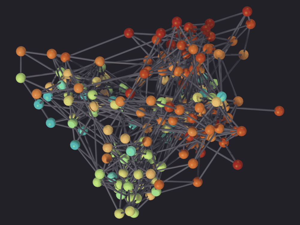
Below: the run at seed 1234, colored by how far each node ended up from where seed 99 put it, after alignment. The top 2 % is clipped, as everywhere in this suite.

draw(graph, "renders/14_layouts/2_seed_residual",
     look='ink', color_attribute="node_shift", clip_high_pct=98)

Info: Geometry Nodes modifier added
Info: Attribute -> node_shift  ·  node_shift -> turbo [log]  [0.02009 … 1.505] on Point

[PASS] 2_seed_residual.png legible — 33.2% ink (healthy range 0.5–60%)

The caption has to be checked against the numbers: the first one written for this figure was wrong. It said the block interiors barely move and the residual concentrates on the nodes bridging two blocks, which is what the picture looks like and a plausible story (a node with fewer ties has less telling it where to go). It is not what the data says.

loyalty = np.array([
                   sum(1 for v in G.neighbors(u) if block[v] == block[u]) / max(G.degree(u), 1)
                   for u in G.nodes()])
bridging = loyalty < np.median(loyalty)

print(f"residual vs in-block neighbor fraction  : "
      f"{np.corrcoef(residual, loyalty)[0, 1]:+.3f}")
print(f"residual vs degree                      : "
      f"{np.corrcoef(residual, degree)[0, 1]:+.3f}")
print(f"median residual, bridging nodes         : "
      f"{np.median(residual[bridging]):.3f}")
print(f"median residual, block-interior nodes   : "
      f"{np.median(residual[~bridging]):.3f}")

check("the residual is not concentrated on the bridging nodes",
      np.median(residual[bridging]) <= np.median(residual[~bridging]),
      "the opposite of what the figure appears to show")

residual vs in-block neighbor fraction  : +0.181
residual vs degree                      : -0.134
median residual, bridging nodes         : 0.483
median residual, block-interior nodes   : 0.509
[PASS] the residual is not concentrated on the bridging nodes — the opposite of what the figure appears to show

True

The two medians differ by five percent, in the other direction: a bridging node moves marginally less than one inside a block. Neither correlation printed above reaches 0.2 in absolute value, a few per cent of the variance between them. The only one pointing somewhere sensible is degree, which is negative: a node with more edges is more constrained and settles in more nearly the same place.

What the eye reads as structure is a smooth gradient across the frame, which is what an alignment residual looks like when a rigid rotation has been removed from something that was not related by one. An artifact of the comparison, not a property of the nodes. The figure is kept because a colored field can look organized, support a sentence that sounds right, and mean nothing.

3.3 · What survives the seed

If the picture moves and the relations do not, measure the relations: the mean distance between two nodes of the same block divided by the mean distance between two nodes of different blocks. Below 1 means the layout put the blocks together; 1 means it did not.

def block_ratio(pos, groups):
    """Within-group over between-group mean distance, on unit-RMS positions."""
    pos = unit(pos)
    d = np.linalg.norm(pos[:, None, :] - pos[None, :, :], axis=-1)
    same = groups[:, None] == groups[None, :]
    np.fill_diagonal(same, False)
    return float(d[same].mean() / d[~same].mean())


for seed, pos in seeded.items():
    print(f"pipeline seed {seed:<6} block ratio {block_ratio(pos, block):.3f}")

ratios = [block_ratio(pos, block) for pos in seeded.values()]
check("the finding survives the seed even though the figure does not",
      abs(ratios[0] - ratios[1]) < 0.02,
      f"{ratios[0]:.3f} vs {ratios[1]:.3f}")

pipeline seed 1234   block ratio 0.451
pipeline seed 99     block ratio 0.447
[PASS] the finding survives the seed even though the figure does not — 0.451 vs 0.447

True

The rule for seeds: quote the measurement, publish the seed, and do not build an argument on the shape of the picture. Two runs of the same force layout agree on the answer to four decimal places and disagree about where everything is.

4 · Seven layouts, one graph

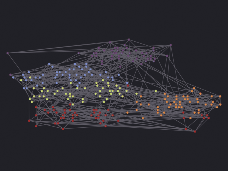
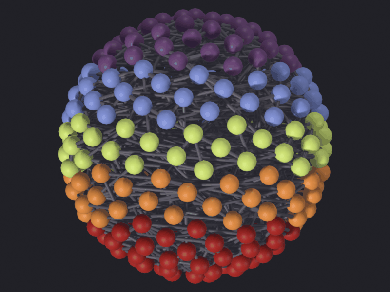
Everything except the algorithm is held fixed: the same object, the same 240 nodes and 840 edges, scale=5.0 and iterations=100, the same look, attribute and camera. Each run overwrites the previous one’s positions on the same mesh, so nothing else can have drifted between panels. One per family, plus two controls:

panel	family	what it optimizes
RANDOM	geometric	nothing; the control
IGRAPH_FR	force-directed	edge length against node repulsion, in 3D
YIFAN_HU	force-directed, multilevel	the same, coarsened (Graphviz sfdp)
IGRAPH_KK	stress	drawn distance against graph distance
SPECTRAL_3D	spectral	the Laplacian’s low eigenvectors
GRAPHVIZ_DOT	hierarchical	layers, then crossings within a layer
SPHERE	geometric	nothing; node i goes to point i of a Fibonacci sphere

Four numbers go with each panel: extent and median NN, the size of the result and the typical spacing inside it in Blender units (why the node radius is re-derived per panel); block ratio, the measure from section 3.3; and hidden, the fraction of nodes a top-down view puts behind another node (section 6).

def plan_occlusion(pos, radius):
    """Fraction of nodes covered by a nearer one in a top-down projection."""
    order = np.argsort(-pos[:, 2])
    xy = pos[:, :2]
    hidden = 0
    for rank in range(1, len(order)):
        node = order[rank]
        above = order[:rank]
        if (np.linalg.norm(xy[above] - xy[node], axis=1) < radius).any():
            hidden += 1
    return hidden / len(pos)


def z_share(pos):
    """Share of the layout's spread carried by its third principal axis."""
    pos = pos - pos.mean(axis=0)
    singular = np.linalg.svd(pos, full_matrices=False)[1]
    return float(singular[2] / singular.sum())


PANELS = ['RANDOM', 'IGRAPH_FR', 'YIFAN_HU', 'IGRAPH_KK', 'SPECTRAL_3D',
          'GRAPHVIZ_DOT', 'SPHERE']

panel_stats = {}
for algorithm in PANELS:
    pos, elapsed = apply(graph, algorithm)
    if pos is None:
        print(f"{algorithm}: did not finish")
        continue
    (_center, _size, diagonal, median_nn), _source = sg.render.measure(graph)
    radius = median_nn * sg.render.NODE_FRACTION
    panel_stats[algorithm] = {
        "seconds": elapsed, "extent": diagonal, "median_nn": median_nn,
        "radius": radius, "ratio": block_ratio(pos, block),
        "hidden": plan_occlusion(pos, radius), "z_share": z_share(pos),
    }
    print(f"{algorithm}  {elapsed:.2f} s")
    draw(graph, f"renders/14_layouts/3_{algorithm.lower()}",
         resolution=(800, 600), width=700,
         look='ink', color_attribute="node_block")

======================================================================
Layout algorithm: RANDOM
Graph: 240 nodes, 840 edges
Parameters:
  - algorithm: RANDOM
  - iterations: 100
  - scale: 5.0000
  - num_nodes: 240
  - num_edges: 840
Execution time: 0.001s
Status: success
======================================================================

Info: Layout 'RANDOM' applied
RANDOM  0.00 s
Info: Geometry Nodes modifier added
Info: Attribute -> node_block  ·  node_block -> turbo [log]  [0 … 4] on Point

[PASS] 3_random.png legible — 56.0% ink (healthy range 0.5–60%)
Computing igraph Fruchterman-Reingold layout for 240 nodes...
  Fruchterman-Reingold completed in 0.01s

======================================================================
Layout algorithm: IGRAPH_FR
Graph: 240 nodes, 840 edges
Parameters:
  - algorithm: IGRAPH_FR
  - iterations: 100
  - scale: 5.0000
  - num_nodes: 240
  - num_edges: 840
Execution time: 0.012s
Status: success
======================================================================

Info: Layout 'IGRAPH_FR' applied
IGRAPH_FR  0.02 s
Info: Geometry Nodes modifier added
Info: Attribute -> node_block  ·  node_block -> turbo [log]  [0 … 4] on Point

[PASS] 3_igraph_fr.png legible — 30.2% ink (healthy range 0.5–60%)
Computing Yifan Hu layout for 240 nodes...
  mode=2Z, backend=scigraphs-utils, engine=sfdp
  z_method=SPECTRAL, z_scale=0.30000001192092896
  Generated Graphviz Z via SPECTRAL: -0.750 to 0.212
  scigraphs-utils Graphviz sfdp computed 240 nodes
  Z range: -0.750 to 0.212
  Final ranges (scale=5.0): X=5.0, Y=4.8, Z=1.0
  Yifan Hu (scigraphs-utils sfdp, mode=2Z) completed in 0.04s

======================================================================
Layout algorithm: YIFAN_HU
Graph: 240 nodes, 840 edges
Parameters:
  - algorithm: YIFAN_HU
  - iterations: 100
  - scale: 5.0000
  - num_nodes: 240
  - num_edges: 840
Execution time: 0.037s
Status: success
======================================================================

Info: Layout 'YIFAN_HU' applied
YIFAN_HU  0.04 s
Info: Geometry Nodes modifier added
Info: Attribute -> node_block  ·  node_block -> turbo [log]  [0 … 4] on Point

[PASS] 3_yifan_hu.png legible — 26.6% ink (healthy range 0.5–60%)
Computing igraph Kamada-Kawai layout for 240 nodes...
  Kamada-Kawai completed in 0.05s

======================================================================
Layout algorithm: IGRAPH_KK
Graph: 240 nodes, 840 edges
Parameters:
  - algorithm: IGRAPH_KK
  - iterations: 100
  - scale: 5.0000
  - num_nodes: 240
  - num_edges: 840
Execution time: 0.057s
Status: success
======================================================================

Info: Layout 'IGRAPH_KK' applied
IGRAPH_KK  0.06 s
Info: Geometry Nodes modifier added
Info: Attribute -> node_block  ·  node_block -> turbo [log]  [0 … 4] on Point

[PASS] 3_igraph_kk.png legible — 38.1% ink (healthy range 0.5–60%)
Computing Spectral 3D layout for 240 nodes...
  Spectral 3D completed in 0.03s

======================================================================
Layout algorithm: SPECTRAL_3D
Graph: 240 nodes, 840 edges
Parameters:
  - algorithm: SPECTRAL_3D
  - iterations: 100
  - scale: 5.0000
  - num_nodes: 240
  - num_edges: 840
Execution time: 0.034s
Status: success
======================================================================

Info: Layout 'SPECTRAL_3D' applied
SPECTRAL_3D  0.04 s
Info: Geometry Nodes modifier added
Info: Attribute -> node_block  ·  node_block -> turbo [log]  [0 … 4] on Point

[PASS] 3_spectral_3d.png legible — 2.1% ink (healthy range 0.5–60%)
  scigraphs-utils Graphviz dot computed 240 nodes

======================================================================
Layout algorithm: GRAPHVIZ_DOT
Graph: 240 nodes, 840 edges
Parameters:
  - algorithm: GRAPHVIZ_DOT
  - iterations: 100
  - scale: 5.0000
  - num_nodes: 240
  - num_edges: 840
Execution time: 0.446s
Status: success
======================================================================

Info: Layout 'GRAPHVIZ_DOT' applied
GRAPHVIZ_DOT  0.45 s
Info: Geometry Nodes modifier added
Info: Attribute -> node_block  ·  node_block -> turbo [log]  [0 … 4] on Point

[PASS] 3_graphviz_dot.png legible — 23.9% ink (healthy range 0.5–60%)

======================================================================
Layout algorithm: SPHERE
Graph: 240 nodes, 840 edges
Parameters:
  - algorithm: SPHERE
  - iterations: 100
  - scale: 5.0000
  - num_nodes: 240
  - num_edges: 840
Execution time: 0.001s
Status: success
======================================================================

Info: Layout 'SPHERE' applied
SPHERE  0.01 s
Info: Geometry Nodes modifier added
Info: Attribute -> node_block  ·  node_block -> turbo [log]  [0 … 4] on Point

[PASS] 3_sphere.png legible — 48.7% ink (healthy range 0.5–60%)

print(f"{'algorithm':<14}{'s':>7}{'extent':>9}{'median NN':>11}"
      f"{'radius':>9}{'block ratio':>13}{'hidden':>8}{'z share':>9}")
print("-" * 80)
for algorithm, s in panel_stats.items():
    print(f"{algorithm:<14}{s['seconds']:7.2f}{s['extent']:9.2f}"
          f"{s['median_nn']:11.4f}{s['radius']:9.4f}{s['ratio']:13.3f}"
          f"{s['hidden']:8.3f}{s['z_share']:9.3f}")

check("the random control finds no structure",
      abs(panel_stats['RANDOM']['ratio'] - 1.0) < 0.05,
      f"block ratio {panel_stats['RANDOM']['ratio']:.3f}")
check("the force layouts do",
      panel_stats['IGRAPH_FR']['ratio'] < 0.6
      and panel_stats['YIFAN_HU']['ratio'] < 0.6)

algorithm           s   extent  median NN   radius  block ratio  hidden  z share
--------------------------------------------------------------------------------
RANDOM           0.00     8.59     0.4560   0.1596        1.003   0.275    0.304
IGRAPH_FR        0.02   125.04     5.2033   1.8212        0.448   0.267    0.291
YIFAN_HU         0.04     6.99     0.1562   0.0547        0.493   0.000    0.035
IGRAPH_KK        0.06   132.87     6.7399   2.3590        0.527   0.354    0.312
SPECTRAL_3D      0.04     7.52     0.0366   0.0128        0.373   0.192    0.333
GRAPHVIZ_DOT     0.45     5.45     0.0779   0.0273        0.507   0.000    0.000
SPHERE           0.01    17.27     1.1024   0.3858        0.753   0.362    0.333
[PASS] the random control finds no structure — block ratio 1.003
[PASS] the force layouts do

True

Is the color keeping up?

sg.render.material() declines to overwrite an existing <obj>_SciGraphsColor material (notebooks/tools/sg.render.py:736-740) and rewires whichever color layer it finds (:759-765), so an object colored once can keep that coloring through a later render that asked for a different attribute. nb.ink() cannot see the difference, because the same nodes are lit either way.

The panels above all use one attribute; the risk is in the rest of the notebook, which recolors this same object by node_shift, node_late_move and node_degree in turn. Two renders of one layout under two attributes, compared pixel by pixel, settle it.

apply(graph, 'IGRAPH_FR')
margin = framing_margin(graph, (400, 300))
by_block = nb.render(
    graph, "renders/14_layouts/_color_check_block", resolution=(400, 300),
    look='ink', color_attribute="node_block", margin=margin,
    shrink=False, verbose=False)
by_degree = nb.render(
    graph, "renders/14_layouts/_color_check_degree", resolution=(400, 300),
    look='ink', color_attribute="node_degree", margin=margin,
    shrink=False, verbose=False)

changed = sg.render.differing_fraction(by_degree, by_block)
ink_block, ink_degree = nb.ink(by_block), nb.ink(by_degree)
print(f"ink, colored by block  : {ink_block:.4f}")
print(f"ink, colored by degree : {ink_degree:.4f}   "
      f"(apart by {abs(ink_block - ink_degree) / ink_block:.1%}; the same "
      f"nodes are lit either way, so this cannot be the check)")
print(f"pixels that actually changed color: {changed:.1%}")

check("the graph really is recolored between renders",
      changed > 0.05,
      "a stale material would leave this near zero while every other "
      "number in the render stayed healthy")

Computing igraph Fruchterman-Reingold layout for 240 nodes...
  Fruchterman-Reingold completed in 0.01s

======================================================================
Layout algorithm: IGRAPH_FR
Graph: 240 nodes, 840 edges
Parameters:
  - algorithm: IGRAPH_FR
  - iterations: 100
  - scale: 5.0000
  - num_nodes: 240
  - num_edges: 840
Execution time: 0.011s
Status: success
======================================================================

Info: Layout 'IGRAPH_FR' applied
Info: Geometry Nodes modifier added
Info: Attribute -> node_block  ·  node_block -> turbo [log]  [0 … 4] on Point
Info: Geometry Nodes modifier added
Info: Attribute -> node_degree  ·  node_degree -> turbo [log]  [1 … 14] on Point
ink, colored by block  : 0.4175
ink, colored by degree : 0.4189   (apart by 0.3%; the same nodes are lit either way, so this cannot be the check)
pixels that actually changed color: 17.1%
[PASS] the graph really is recolored between renders — a stale material would leave this near zero while every other number in the render stayed healthy

True

Reading the panels

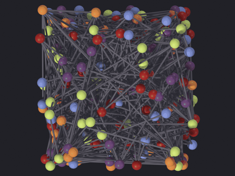
The control is the densest figure here. RANDOM reaches 57 % ink, three points under the ceiling check_render allows, and its block ratio is 1.003: the groups are neither together nor apart. Everything the other six panels show, they added.

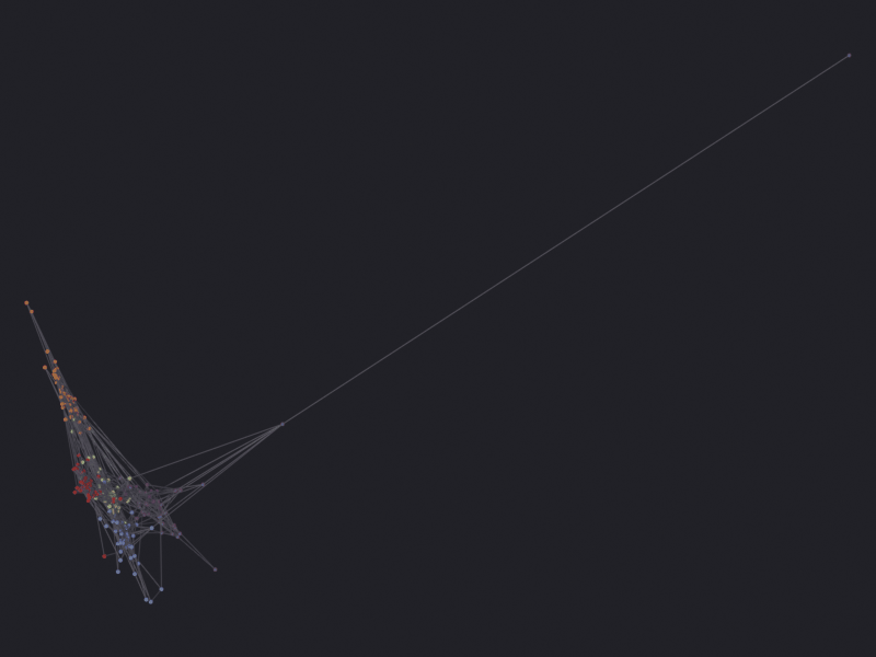
scale=5.0 does not mean the same thing twice. Extents run from 5.4 Blender units (GRAPHVIZ_DOT) to 140 (IGRAPH_FR, IGRAPH_KK), a factor of twenty-six; median spacing from 0.037 to 6.7, a factor of a hundred and eighty. The Graphviz and geometric layouts normalize to the requested scale; the igraph ones multiply igraph’s own output by it (igraph_layouts.py:37, :70), and that output is whatever its simulation reached. Hence a scale slider with no visible effect, and a node radius derived per panel: at a fixed radius, five of these seven are either a solid mat or a field of specks.

SPECTRAL_3D spends the whole frame on one node. Its block ratio is the best of the seven at 0.373 and its figure is nearly empty: nx.spectral_layout normalizes by the extreme coordinate, one node sits far out on the second eigenvector, and the rest are compressed into a corner. The median nearest-neighbor distance is 0.037 against an extent of 7.5, a ratio of 1:205, where the force layouts sit near 1:27. Both readings are correct: spectral embedding does separate the blocks, and does put almost all of them in one small region.

SPHERE scores 0.753 without reading a single edge, showing the five blocks as five clean bands. A Fibonacci sphere places node i by its index and the nodes were numbered in block order, so the blocks are contiguous in index. Change the numbering and the bands vanish while the graph stays identical. A structure score below 1 is not by itself evidence of structure.

shuffled = np.random.default_rng(0).permutation(len(block))
pos_sphere, _ = apply(graph, 'SPHERE')
print(f"SPHERE, blocks as numbered : {block_ratio(pos_sphere, block):.3f}")
print(f"SPHERE, blocks relabeled   : "
      f"{block_ratio(pos_sphere, block[shuffled]):.3f}")
print(f"IGRAPH_FR, blocks relabeled : "
      f"{block_ratio(apply(graph, 'IGRAPH_FR')[0], block[shuffled]):.3f}")

check("SPHERE's score is an artifact of the node numbering",
      block_ratio(pos_sphere, block[shuffled]) > 0.95,
      "relabeling the nodes destroys it and leaves the graph untouched")

======================================================================
Layout algorithm: SPHERE
Graph: 240 nodes, 840 edges
Parameters:
  - algorithm: SPHERE
  - iterations: 100
  - scale: 5.0000
  - num_nodes: 240
  - num_edges: 840
Execution time: 0.002s
Status: success
======================================================================

Info: Layout 'SPHERE' applied
SPHERE, blocks as numbered : 0.753
SPHERE, blocks relabeled   : 0.997
Computing igraph Fruchterman-Reingold layout for 240 nodes...
  Fruchterman-Reingold completed in 0.01s

======================================================================
Layout algorithm: IGRAPH_FR
Graph: 240 nodes, 840 edges
Parameters:
  - algorithm: IGRAPH_FR
  - iterations: 100
  - scale: 5.0000
  - num_nodes: 240
  - num_edges: 840
Execution time: 0.012s
Status: success
======================================================================

Info: Layout 'IGRAPH_FR' applied
IGRAPH_FR, blocks relabeled : 1.005
[PASS] SPHERE's score is an artifact of the node numbering — relabeling the nodes destroys it and leaves the graph untouched

True

5 · One step at a time

A force layout is an iteration, and apply_layout hides that: it runs the whole thing and hands back the fixed point. scigraphs.execute_layout_step advances the simulation one timeline frame at a time and keyframes as it goes, which is how the Gephi-style panel animates a layout settling.

That operator is modal: it installs a window-manager timer and a modal handler, so it needs a window and cannot run under blender -b at all. It is also not what does the arithmetic. The function underneath, layout.execute_layout_iteration(obj, ...), is plain Python, touches only the object, and returns (success, energy); called once per step below.

determinism.set_pipeline_seed(7)
start_positions = np.random.default_rng(7).random((graph["num_nodes"], 3)) * 5.0
graph["node_positions"] = start_positions.flatten().tolist()
graph["layout_iteration"] = 0

STEPS = 60
history = []
started = time.time()
with nb.quiet():
    for step in range(STEPS):
        before = positions(graph)
        ok, energy = sglayout.execute_layout_iteration(
            graph, algorithm='SPRING_3D', scale=5.0, current_frame=step)
        moved = np.linalg.norm(positions(graph) - before, axis=1)
        history.append((step + 1, float(energy), float(moved.sum()),
                       float(moved.max()), bool(ok)))
elapsed = time.time() - started
determinism.set_pipeline_seed(None)

print(f"{STEPS} steps on {graph['num_nodes']} nodes in {elapsed:.1f} s "
      f"({elapsed / STEPS * 1000:.0f} ms per step)")
print()
print(f"{'step':>5}{'energy':>14}{'total moved':>14}{'largest move':>14}")
print("-" * 47)
for row in history[:3] + history[4::10] + [history[-1]]:
    print(f"{row[0]:>5}{row[1]:>14.1f}{row[2]:>14.3f}{row[3]:>14.4f}")

======================================================================
Layout algorithm: SPRING_3D
Graph: 240 nodes, 840 edges
Parameters:
  - mode: INTERACTIVE
  - iteration: 0
  - frame: 0
  - scale: 5.0000
  - energy: 32074.2833
  - energy_change: 0.0000
  - repulsion: 1.0000
  - attraction: 1.0000
  - gravity: 0.1000
  - cooling: 0.9500
  - initial_temp: 1.0000
  - edge_dist: 1.0000
Execution time: 0.111s
Status: success
======================================================================


======================================================================
Layout algorithm: SPRING_3D
Graph: 240 nodes, 840 edges
Parameters:
  - mode: INTERACTIVE
  - iteration: 50
  - frame: 50
  - scale: 5.0000
  - energy: 4199.2942
  - energy_change: 19.5934
  - repulsion: 1.0000
  - attraction: 1.0000
  - gravity: 0.1000
  - cooling: 0.9500
  - initial_temp: 1.0000
  - edge_dist: 1.0000
Execution time: 0.111s
Status: success
======================================================================

60 steps on 240 nodes in 6.6 s (110 ms per step)

 step        energy   total moved  largest move
-----------------------------------------------
    1       32074.3       240.000        1.0000
    2       13220.5       228.000        0.9500
    3        6238.5       216.600        0.9025
    5        5604.0       195.481        0.8145
   15        4771.0       117.042        0.4877
   25        4390.0        70.077        0.2920
   35        4258.9        41.958        0.1748
   45        4213.1        25.122        0.1047
   55        4195.4        15.041        0.0627
   60        4174.9        11.639        0.0485

The energy (the quantity the operator reports and auto-stops on, a sum of force magnitudes rather than an energy in any physical sense) falls by 81 % over the first five steps and by 26 % over the remaining fifty-five. Almost all of the layout happens immediately, and the rest is refinement. Cutting a 100-iteration run to 20 changes the figure much less than the iteration count suggests; cutting it to 5 changes it a great deal.

The two movement columns say nothing at all. Every node moves exactly the same distance on every step, and that distance is the annealing temperature: _spring_iteration_advanced normalizes each force to a unit vector and multiplies by min(|force|, temperature) (SciGraphs/core/mesh/layouts/interactive.py:395), and here the forces are four orders of magnitude larger than the temperature, so the minimum is always the temperature. Total movement per step is therefore n × initial_temperature × cooling_factor ** step, a geometric decay that would be nearly identical on a different graph or with no edges at all. The largest single move matches the temperature exactly at every step; the total is within a couple of percent of n times it, the gap being the few nodes whose force falls below the temperature late in the run.

predicted = [graph["num_nodes"] * 1.0 * 0.95 ** step for step in range(STEPS)]
observed = [row[2] for row in history]
error = max(abs(p - o) / p for p, o in zip(predicted, observed))
print(f"total movement per step, predicted from the cooling schedule alone "
      f"with no reference to the graph: worst error {error * 100:.2f}%")
print(f"largest single move at step 1 / step {STEPS}: "
      f"{history[0][3]:.4f} / {history[-1][3]:.4f}   "
      f"(0.95 ** {STEPS - 1} = {0.95 ** (STEPS - 1):.4f}, exactly)")

check("per-step movement is the cooling schedule and nothing else",
      error < 0.03,
      "it is not a convergence signal; read the energy instead")

total movement per step, predicted from the cooling schedule alone with no reference to the graph: worst error 0.30%
largest single move at step 1 / step 60: 1.0000 / 0.0485   (0.95 ** 59 = 0.0485, exactly)
[PASS] per-step movement is the cooling schedule and nothing else — it is not a convergence signal; read the energy instead

True

So the stopping rule has to be built on the energy, which is what auto_stop_threshold in the panel compares against: it stops when the change in energy between two steps falls below the threshold (interactive.py:279-282).

initial = history[0][1]
changes = [(row[0], abs(row[1] - previous[1]))
           for previous, row in zip(history, history[1:])]
settled = next((step for step, change in changes
               if change < 0.01 * history[step - 1][1]), None)
print(f"energy at step 1  : {initial:.1f}")
print(f"energy at step {STEPS} : {history[-1][1]:.1f} "
      f"({history[-1][1] / initial * 100:.1f}% of the first step)")
print(f"first step whose energy change is under 1%: {settled}")

check("the layout converges rather than oscillating",
      history[-1][1] < history[0][1] and changes[-1][1] < changes[0][1])

energy at step 1  : 32074.3
energy at step 60 : 4174.9 (13.0% of the first step)
first step whose energy change is under 1%: 10
[PASS] the layout converges rather than oscillating

True

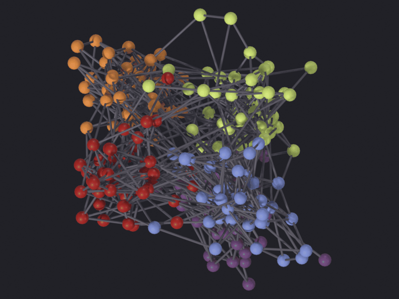
The figure: the same graph, colored by the net displacement of each node over the last twenty steps, where it ended up against where it was, not the distance traveled getting there. Every node covers the same ground per step, so a node still being pulled somewhere shows a large net displacement and a node pushed back and forth between two neighbors shows almost none. It shows where the layout has not finished deciding, which is otherwise only visible in an animation.

tail = positions(graph)
with nb.quiet():
    for step in range(20):
        sglayout.execute_layout_iteration(graph, algorithm='SPRING_3D',
                                          scale=5.0, current_frame=STEPS + step)
put_attribute(graph, "node_late_move",
              np.linalg.norm(positions(graph) - tail, axis=1))

'node_late_move'

Add-on defect: the step operator leaves the mesh animated, and the next render draws the wrong frame. execute_layout_iteration inserts a keyframe on the object’s location and on every vertex’s co at current_frame (SciGraphs/core/mesh/layouts/interactive.py:296-300). From then on the mesh is driven by an action, so the geometry a render draws is the pose at the scene’s current frame (frame 1, unless something moved it) while everything that reads obj["node_positions"], including the camera fit, sees the final positions. The figure comes out framed on one layout and drawn from another, a small blob in the corner of a frame sized for something else. scigraphs.reset_layout clears the animation data, which is the half of that operator worth having; cleared explicitly here.

def mesh_drift(obj):
    """How far the drawn mesh has got from `node_positions`, in Blender units.

    `frame_set` rather than `view_layer.update()`, and that distinction is why
    this is a silent failure: an update does not re-evaluate the action, so the
    mesh reads correct until something does (a frame change, or a render).
    Measured on this graph: 0.0 after the update, four Blender units after the
    frame is set to the frame it was already on.
    """
    scene = bpy.context.scene
    scene.frame_set(scene.frame_current)
    mesh = np.empty(len(obj.data.vertices) * 3, dtype=np.float32)
    obj.data.vertices.foreach_get("co", mesh)
    return float(np.abs(positions(obj) - mesh.reshape(-1, 3)).max())


animated = (graph.animation_data is not None,
            graph.data.animation_data is not None)
drift_before = mesh_drift(graph)

if graph.animation_data:
    graph.animation_data_clear()
if graph.data.animation_data:
    graph.data.animation_data_clear()
geometry.update_node_positions_from_property(graph)
geometry.rebuild_edges(graph)

drift_after = mesh_drift(graph)
print(f"animation left on (object, mesh) : {animated}")
print(f"property vs drawn mesh, before   : {drift_before:.3f} Blender units")
print(f"                        after    : {drift_after:.3f}")

check("the mesh agrees with the positions again",
      drift_after < 1e-5,
      "without this the render is framed on one layout and drawn from "
      "another")

draw(graph, "renders/14_layouts/4_late_movement",
     look='ink', color_attribute="node_late_move", clip_high_pct=98)

animation left on (object, mesh) : (True, True)
property vs drawn mesh, before   : 4.123 Blender units
                        after    : 0.000
[PASS] the mesh agrees with the positions again — without this the render is framed on one layout and drawn from another
Info: Geometry Nodes modifier added
Info: Attribute -> node_late_move  ·  node_late_move -> turbo [log]  [0.01183 … 0.141] on Point

[PASS] 4_late_movement.png legible — 26.6% ink (healthy range 0.5–60%)

Before you reach for the animated version. execute_layout_iteration’s spring branch is a Python double loop over all node pairs, so it is quadratic and interpreted: 60 steps on 240 nodes took the time printed above, and the cost goes as the square of the node count. SciGraphs/core/mesh/layouts/simulation.py is the vectorized replacement, a ForceSim that keeps its state in NumPy arrays, splits repulsion into an exact near field and a gridded far field, and can be stepped the same way. Its step() returns total displacement rather than an energy: displacement is what the adaptive integrator already computes and what a viewer sees.

from scigraphs_core.mesh.layouts import simulation

edges = np.array(list(G.edges()), dtype=np.int64)
sim = simulation.ForceSim(simulation.random_positions(G.number_of_nodes(),
                          scale=5.0, seed=7),
                          edges, seed=7, scale=5.0)
started = time.time()
trace = [(sim.iteration + 10, sim.step(10)) for _ in range(6)]
sim_elapsed = time.time() - started
print(f"ForceSim: {STEPS} steps in {sim_elapsed:.3f} s, against "
      f"{elapsed:.1f} s for the same {STEPS} steps through the operator's own "
      f"path ({elapsed / max(sim_elapsed, 1e-6):.0f}x)")
for iteration, moved in trace:
    print(f"   iteration {iteration:>3}   moved {moved:8.2f}")

check("the vectorized simulator converges too",
      trace[-1][1] < trace[0][1] / 3,
      "and its movement per step is a real signal, not a cooling curve")

ForceSim: 60 steps in 0.024 s, against 6.6 s for the same 60 steps through the operator's own path (271x)
   iteration  10   moved   152.94
   iteration  20   moved    55.61
   iteration  30   moved    30.75
   iteration  40   moved    16.71
   iteration  50   moved    13.04
   iteration  60   moved    11.56
[PASS] the vectorized simulator converges too — and its movement per step is a real signal, not a cooling curve

True

6 · 2D against 3D

Every figure in this suite is a top-down orthographic plan. That is the right default for a map (notebook 13 sets out why) but it means a 3D layout is being projected, and the projection is not free: two nodes at the same (x, y) and different z are drawn on top of each other, and the axis the layout worked hardest to use is the one the camera throws away. The hidden column of the panel table is that cost measured, at the radius each panel is drawn with.

print(f"{'algorithm':<14}{'z share':>9}{'hidden in plan':>16}")
print("-" * 40)
for algorithm, s in sorted(panel_stats.items(), key=lambda kv: kv[1]['hidden']):
    print(f"{algorithm:<14}{s['z_share']:9.3f}{s['hidden']:>15.1%}")

flat = [a for a, s in panel_stats.items() if s['z_share'] < 0.05]
deep = [a for a, s in panel_stats.items() if s['hidden'] > 0.25]
print(f"\nessentially flat : {', '.join(flat)}")
print(f"over a quarter of the nodes hidden : {', '.join(deep)}")

algorithm       z share  hidden in plan
----------------------------------------
YIFAN_HU          0.035           0.0%
GRAPHVIZ_DOT      0.000           0.0%
SPECTRAL_3D       0.333          19.2%
IGRAPH_FR         0.291          26.7%
RANDOM            0.304          27.5%
IGRAPH_KK         0.312          35.4%
SPHERE            0.333          36.2%

essentially flat : YIFAN_HU, GRAPHVIZ_DOT
over a quarter of the nodes hidden : RANDOM, IGRAPH_FR, IGRAPH_KK, SPHERE

FORCEATLAS2 is not in that table but is the add-on’s scene default, the one the panel offers before anything has been chosen, and it is three-dimensional: the default path produces a layout whose third axis a top-down figure throws away.

pos_fa2, _ = apply(graph, 'FORCEATLAS2')
span = pos_fa2.max(axis=0) - pos_fa2.min(axis=0)
(_c, _s, _d, nn_fa2), _src = sg.render.measure(graph)
print(f"FORCEATLAS2 span   X {span[0]:.2f}  Y {span[1]:.2f}  Z {span[2]:.2f}")
print(f"  the discarded axis is {span[2] / span[:2].max() * 100:.0f}% "
      f"of the longest axis the camera keeps")
print(f"  z share {z_share(pos_fa2):.3f}, "
      f"hidden in plan {plan_occlusion(pos_fa2, nn_fa2 * sg.render.NODE_FRACTION):.1%}")
print(f"  block ratio  3D {block_ratio(pos_fa2, block):.3f}   "
      f"flattened {block_ratio(np.column_stack([pos_fa2[:, :2], np.zeros(len(pos_fa2))]), block):.3f}")

Computing ForceAtlas2 (3D, networkx) for 240 nodes...
  ForceAtlas2 completed in 0.18s

======================================================================
Layout algorithm: FORCEATLAS2
Fallback: using SPRING (2D fallback) instead
   Reason: FORCEATLAS2 library not available
Graph: 240 nodes, 840 edges
Parameters:
  - algorithm: FORCEATLAS2
  - iterations: 100
  - scale: 5.0000
  - num_nodes: 240
  - num_edges: 840
Execution time: 0.184s
Status: success (with fallback)
======================================================================

Info: Layout 'FORCEATLAS2' applied
FORCEATLAS2 span   X 9.19  Y 7.26  Z 8.01
  the discarded axis is 87% of the longest axis the camera keeps
  z share 0.287, hidden in plan 28.7%
  block ratio  3D 0.365   flattened 0.369

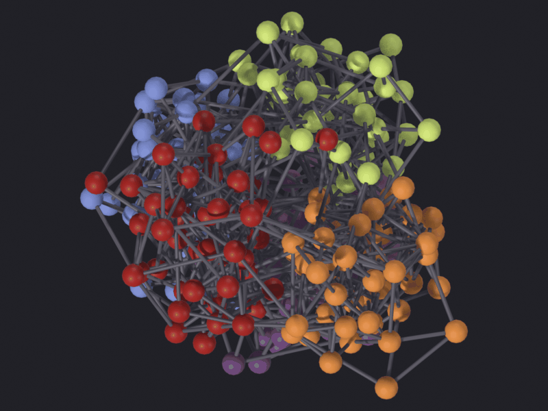
IGRAPH_KK hides 35 % of its nodes and GRAPHVIZ_DOT none, and the difference is entirely the third axis: dot is planar (z share 0.000), YIFAN_HU in its default 2Z mode nearly so (0.031), and the genuinely three-dimensional layouts sit near 0.3. In the Kamada-Kawai panel one entire block is drawn underneath its neighbor and does not appear in the figure at all.

When is a 3D layout worth it? When the extra axis buys separation the plane cannot give, which is measurable: compare each layout’s block ratio against that of its projection onto z = 0, which is what the reader of a plan sees.

print(f"{'algorithm':<14}{'ratio in 3D':>13}{'ratio in plan':>15}{'cost':>8}")
print("-" * 52)
for algorithm in PANELS:
    pos, _ = apply(graph, algorithm)
    if pos is None:
        continue
    flat_pos = pos.copy()
    flat_pos[:, 2] = 0.0
    r3, r2 = block_ratio(pos, block), block_ratio(flat_pos, block)
    print(f"{algorithm:<14}{r3:13.3f}{r2:15.3f}{r2 - r3:+8.3f}")

algorithm       ratio in 3D  ratio in plan    cost
----------------------------------------------------

======================================================================
Layout algorithm: RANDOM
Graph: 240 nodes, 840 edges
Parameters:
  - algorithm: RANDOM
  - iterations: 100
  - scale: 5.0000
  - num_nodes: 240
  - num_edges: 840
Execution time: 0.001s
Status: success
======================================================================

Info: Layout 'RANDOM' applied
RANDOM                1.003          1.005  +0.003
Computing igraph Fruchterman-Reingold layout for 240 nodes...
  Fruchterman-Reingold completed in 0.01s

======================================================================
Layout algorithm: IGRAPH_FR
Graph: 240 nodes, 840 edges
Parameters:
  - algorithm: IGRAPH_FR
  - iterations: 100
  - scale: 5.0000
  - num_nodes: 240
  - num_edges: 840
Execution time: 0.012s
Status: success
======================================================================

Info: Layout 'IGRAPH_FR' applied
IGRAPH_FR             0.447          0.460  +0.014
Computing Yifan Hu layout for 240 nodes...
  mode=2Z, backend=scigraphs-utils, engine=sfdp
  z_method=SPECTRAL, z_scale=0.30000001192092896
  Generated Graphviz Z via SPECTRAL: -0.750 to 0.212
  scigraphs-utils Graphviz sfdp computed 240 nodes
  Z range: -0.750 to 0.212
  Final ranges (scale=5.0): X=5.0, Y=4.8, Z=1.0
  Yifan Hu (scigraphs-utils sfdp, mode=2Z) completed in 0.04s

======================================================================
Layout algorithm: YIFAN_HU
Graph: 240 nodes, 840 edges
Parameters:
  - algorithm: YIFAN_HU
  - iterations: 100
  - scale: 5.0000
  - num_nodes: 240
  - num_edges: 840
Execution time: 0.038s
Status: success
======================================================================

Info: Layout 'YIFAN_HU' applied
YIFAN_HU              0.493          0.493  -0.000
Computing igraph Kamada-Kawai layout for 240 nodes...
  Kamada-Kawai completed in 0.05s

======================================================================
Layout algorithm: IGRAPH_KK
Graph: 240 nodes, 840 edges
Parameters:
  - algorithm: IGRAPH_KK
  - iterations: 100
  - scale: 5.0000
  - num_nodes: 240
  - num_edges: 840
Execution time: 0.054s
Status: success
======================================================================

Info: Layout 'IGRAPH_KK' applied
IGRAPH_KK             0.527          0.530  +0.003
Computing Spectral 3D layout for 240 nodes...
  Spectral 3D completed in 0.04s

======================================================================
Layout algorithm: SPECTRAL_3D
Graph: 240 nodes, 840 edges
Parameters:
  - algorithm: SPECTRAL_3D
  - iterations: 100
  - scale: 5.0000
  - num_nodes: 240
  - num_edges: 840
Execution time: 0.036s
Status: success
======================================================================

Info: Layout 'SPECTRAL_3D' applied
SPECTRAL_3D           0.373          0.386  +0.013
  scigraphs-utils Graphviz dot computed 240 nodes

======================================================================
Layout algorithm: GRAPHVIZ_DOT
Graph: 240 nodes, 840 edges
Parameters:
  - algorithm: GRAPHVIZ_DOT
  - iterations: 100
  - scale: 5.0000
  - num_nodes: 240
  - num_edges: 840
Execution time: 0.452s
Status: success
======================================================================

Info: Layout 'GRAPHVIZ_DOT' applied
GRAPHVIZ_DOT          0.507          0.507  +0.000

======================================================================
Layout algorithm: SPHERE
Graph: 240 nodes, 840 edges
Parameters:
  - algorithm: SPHERE
  - iterations: 100
  - scale: 5.0000
  - num_nodes: 240
  - num_edges: 840
Execution time: 0.001s
Status: success
======================================================================

Info: Layout 'SPHERE' applied
SPHERE                0.753          0.612  -0.140

The projection costs little on this measure. YIFAN_HU and GRAPHVIZ_DOT lose nothing, having had nothing in Z to lose. The genuinely three-dimensional layouts lose between 0.003 and 0.014, a few percent of the structure they found, against 27 to 35 percent of their nodes hidden behind another one. FORCEATLAS2, the default, throws away an axis 87 % as long as the one the camera keeps and pays 0.004 for it.

SPHERE moves the other way: its ratio improves by 0.14 when flattened, because the projection collapses the far hemisphere onto the near one and the index-ordered bands overlap into something that looks even more grouped. A number that gets better when information is destroyed is measuring the wrong thing, and this is the second time SPHERE has scored well by accident.

So the case for three dimensions is rarely the printed figure: the structure survives the projection nearly intact and a third of the nodes do not. It is the viewport, where the graph can be turned, and the export, where the coordinates are the deliverable. For a plan, sfdp in 2Z mode is the add-on’s compromise: a true 2D layout with a Z derived from the spectrum, so the plan loses nothing and the third axis is there to orbit.

Add-on defect: three layouts build their structure in the wrong plane. Blender’s up axis is Z. _circular_hierarchy_layout writes y = 0 and lays its concentric rings out in XZ (SciGraphs/core/mesh/layouts/hierarchical.py:298-303), so a top-down camera sees a straight line: measured below, a Y extent of exactly zero. _hierarchical_layout_3d (hierarchical.py:66-77), _spiral_layout_3d and _helix_layout (basic.py:57-65, :83-91) use the same Y-up convention for their level or height axis, so their structure is also side-on in a plan.

for algorithm in ('CIRCULAR_HIERARCHY', 'HIERARCHICAL_3D', 'HELIX'):
    pos, _ = apply(graph, algorithm)
    span = pos.max(axis=0) - pos.min(axis=0)
    print(f"{algorithm:<20} X {span[0]:6.2f}   Y {span[1]:6.2f}   "
          f"Z {span[2]:6.2f}")

pos_circ, _ = apply(graph, 'CIRCULAR_HIERARCHY')
check("CIRCULAR_HIERARCHY has no extent at all in the plan's Y axis",
      float(pos_circ[:, 1].max() - pos_circ[:, 1].min()) < 1e-9,
      "a top-down render of it is a line")

Computing Circular Hierarchy layout for 240 nodes...
  Circular Hierarchy layout completed in 0.00s

======================================================================
Layout algorithm: CIRCULAR_HIERARCHY
Graph: 240 nodes, 840 edges
Parameters:
  - algorithm: CIRCULAR_HIERARCHY
  - iterations: 100
  - scale: 5.0000
  - num_nodes: 240
  - num_edges: 840
Execution time: 0.004s
Status: success
======================================================================

Info: Layout 'CIRCULAR_HIERARCHY' applied
CIRCULAR_HIERARCHY   X   9.98   Y   0.00   Z   9.99
Computing Hierarchical 3D layout for 240 nodes...
  Hierarchical 3D completed in 0.00s

======================================================================
Layout algorithm: HIERARCHICAL_3D
Graph: 240 nodes, 840 edges
Parameters:
  - algorithm: HIERARCHICAL_3D
  - iterations: 100
  - scale: 5.0000
  - num_nodes: 240
  - num_edges: 840
Execution time: 0.001s
Status: success
======================================================================

Info: Layout 'HIERARCHICAL_3D' applied
HIERARCHICAL_3D      X   5.00   Y  10.00   Z   5.00

======================================================================
Layout algorithm: HELIX
Graph: 240 nodes, 840 edges
Parameters:
  - algorithm: HELIX
  - iterations: 100
  - scale: 5.0000
  - num_nodes: 240
  - num_edges: 840
Execution time: 0.001s
Status: success
======================================================================

Info: Layout 'HELIX' applied
HELIX                X   3.00   Y  10.00   Z   3.00
Computing Circular Hierarchy layout for 240 nodes...
  Circular Hierarchy layout completed in 0.00s

======================================================================
Layout algorithm: CIRCULAR_HIERARCHY
Graph: 240 nodes, 840 edges
Parameters:
  - algorithm: CIRCULAR_HIERARCHY
  - iterations: 100
  - scale: 5.0000
  - num_nodes: 240
  - num_edges: 840
Execution time: 0.005s
Status: success
======================================================================

Info: Layout 'CIRCULAR_HIERARCHY' applied
[PASS] CIRCULAR_HIERARCHY has no extent at all in the plan's Y axis — a top-down render of it is a line

True

7 · Scale

The growth of layout cost with graph size decides which algorithms are usable. Three sizes, six algorithms, the same Watts-Strogatz construction at each size so the density is held constant.

The graphs are built and thrown away one at a time: a 3,000-node mesh with 9,000 edges is cheap, but leaving three of them in the scene would put them in every subsequent render.

SIZES = (200, 800, 3000)
TIMED = ['SPECTRAL_3D', 'IGRAPH_FR', 'YIFAN_HU', 'GRAPHVIZ_SFDP',
         'IGRAPH_KK', 'SPRING_3D']

# Smallest size only: one `GRAPHVIZ_CIRCO` run on section 4's denser 240-node
# graph takes nearly four minutes, longer than the rest of this notebook
# together.
SLOW = ['CIRCLE_PACKING', 'GRAPHVIZ_CIRCO']

def best_of(obj, algorithm, repeats=3, cheap=2.0):
    """Fastest of a few runs, but only while a run is cheap.

    A single measurement of a layout that takes twenty milliseconds is mostly
    noise: the same call came out at 0.03 s and 0.12 s in two runs of this
    notebook, a factor of four in a growth column trying to show a factor of
    fifteen. The minimum of three removes that; the guard stops the same
    discipline costing ninety seconds where one run is already unambiguous.
    """
    _pos, seconds = apply(obj, algorithm)
    while repeats > 1 and seconds < cheap:
        _pos, again = apply(obj, algorithm)
        seconds = min(seconds, again)
        repeats -= 1
    return seconds


timings = {}
for n in SIZES:
    Gn = nx.connected_watts_strogatz_graph(n, 6, 0.08, seed=3)
    with nb.quiet():
        with bpy.context.temp_override(collection=COLL):
            probe = geometry.create_graph_object(GraphData(list(Gn.nodes()),
                                                 list(Gn.edges())))
    probe.name = f"Scale_{n}"
    for algorithm in TIMED:
        timings[(n, algorithm)] = best_of(probe, algorithm)
    if n == SIZES[0]:
        for algorithm in SLOW:
            timings[(n, algorithm)] = best_of(probe, algorithm)
    bpy.data.objects.remove(probe, do_unlink=True)
    print(f"  {n} nodes done")

print()
header = "".join(f"{n:>12}" for n in SIZES)
print(f"{'algorithm':<16}{header}{'growth':>12}")
print("-" * (16 + 12 * len(SIZES) + 12))
for algorithm in TIMED:
    row = "".join(f"{timings[(n, algorithm)]:>11.2f}s" for n in SIZES)
    first, last = timings[(SIZES[0], algorithm)], timings[(SIZES[-1], algorithm)]
    growth = last / first if first > 1e-4 else float("nan")
    print(f"{algorithm:<16}{row}{growth:>11.0f}x")

print(f"\nthe graph grew {SIZES[-1] / SIZES[0]:.0f}x; "
      f"quadratic cost would be {(SIZES[-1] / SIZES[0]) ** 2:.0f}x")
print(f"\nat {SIZES[0]} nodes only, because one run is more than the rest of "
      f"the table costs together:")
for algorithm in SLOW:
    seconds = timings[(SIZES[0], algorithm)]
    print(f"  {algorithm:<16}{seconds:8.1f}s"
          f"   ({seconds / timings[(SIZES[0], 'GRAPHVIZ_SFDP')]:.0f}x "
          f"GRAPHVIZ_SFDP on the same graph)")

Creating graph object with 200 nodes...
  Random positions generated in 0.00s (seed=1426602425)
  Vertices created in 0.00s
  600 edges created in 0.00s
  Mesh conversion in 0.00s
  Object created in 0.00s
Total graph creation time: 0.00s
Computing Spectral 3D layout for 200 nodes...
  Spectral 3D completed in 0.02s

======================================================================
Layout algorithm: SPECTRAL_3D
Graph: 200 nodes, 600 edges
Parameters:
  - algorithm: SPECTRAL_3D
  - iterations: 100
  - scale: 5.0000
  - num_nodes: 200
  - num_edges: 600
Execution time: 0.021s
Status: success
======================================================================

Info: Layout 'SPECTRAL_3D' applied
Computing Spectral 3D layout for 200 nodes...
  Spectral 3D completed in 0.02s

======================================================================
Layout algorithm: SPECTRAL_3D
Graph: 200 nodes, 600 edges
Parameters:
  - algorithm: SPECTRAL_3D
  - iterations: 100
  - scale: 5.0000
  - num_nodes: 200
  - num_edges: 600
Execution time: 0.021s
Status: success
======================================================================

Info: Layout 'SPECTRAL_3D' applied
Computing Spectral 3D layout for 200 nodes...
  Spectral 3D completed in 0.02s

======================================================================
Layout algorithm: SPECTRAL_3D
Graph: 200 nodes, 600 edges
Parameters:
  - algorithm: SPECTRAL_3D
  - iterations: 100
  - scale: 5.0000
  - num_nodes: 200
  - num_edges: 600
Execution time: 0.021s
Status: success
======================================================================

Info: Layout 'SPECTRAL_3D' applied
Computing igraph Fruchterman-Reingold layout for 200 nodes...
  Fruchterman-Reingold completed in 0.01s

======================================================================
Layout algorithm: IGRAPH_FR
Graph: 200 nodes, 600 edges
Parameters:
  - algorithm: IGRAPH_FR
  - iterations: 100
  - scale: 5.0000
  - num_nodes: 200
  - num_edges: 600
Execution time: 0.009s
Status: success
======================================================================

Info: Layout 'IGRAPH_FR' applied
Computing igraph Fruchterman-Reingold layout for 200 nodes...
  Fruchterman-Reingold completed in 0.01s

======================================================================
Layout algorithm: IGRAPH_FR
Graph: 200 nodes, 600 edges
Parameters:
  - algorithm: IGRAPH_FR
  - iterations: 100
  - scale: 5.0000
  - num_nodes: 200
  - num_edges: 600
Execution time: 0.009s
Status: success
======================================================================

Info: Layout 'IGRAPH_FR' applied
Computing igraph Fruchterman-Reingold layout for 200 nodes...
  Fruchterman-Reingold completed in 0.01s

======================================================================
Layout algorithm: IGRAPH_FR
Graph: 200 nodes, 600 edges
Parameters:
  - algorithm: IGRAPH_FR
  - iterations: 100
  - scale: 5.0000
  - num_nodes: 200
  - num_edges: 600
Execution time: 0.009s
Status: success
======================================================================

Info: Layout 'IGRAPH_FR' applied
Computing Yifan Hu layout for 200 nodes...
  mode=2Z, backend=scigraphs-utils, engine=sfdp
  z_method=SPECTRAL, z_scale=0.30000001192092896
  Generated Graphviz Z via SPECTRAL: -0.555 to 0.750
  scigraphs-utils Graphviz sfdp computed 200 nodes
  Z range: -0.555 to 0.750
  Final ranges (scale=5.0): X=5.0, Y=4.4, Z=1.3
  Yifan Hu (scigraphs-utils sfdp, mode=2Z) completed in 0.03s

======================================================================
Layout algorithm: YIFAN_HU
Graph: 200 nodes, 600 edges
Parameters:
  - algorithm: YIFAN_HU
  - iterations: 100
  - scale: 5.0000
  - num_nodes: 200
  - num_edges: 600
Execution time: 0.031s
Status: success
======================================================================

Info: Layout 'YIFAN_HU' applied
Computing Yifan Hu layout for 200 nodes...
  mode=2Z, backend=scigraphs-utils, engine=sfdp
  z_method=SPECTRAL, z_scale=0.30000001192092896
  Generated Graphviz Z via SPECTRAL: -0.555 to 0.750
  scigraphs-utils Graphviz sfdp computed 200 nodes
  Z range: -0.555 to 0.750
  Final ranges (scale=5.0): X=5.0, Y=4.4, Z=1.3
  Yifan Hu (scigraphs-utils sfdp, mode=2Z) completed in 0.03s

======================================================================
Layout algorithm: YIFAN_HU
Graph: 200 nodes, 600 edges
Parameters:
  - algorithm: YIFAN_HU
  - iterations: 100
  - scale: 5.0000
  - num_nodes: 200
  - num_edges: 600
Execution time: 0.030s
Status: success
======================================================================

Info: Layout 'YIFAN_HU' applied
Computing Yifan Hu layout for 200 nodes...
  mode=2Z, backend=scigraphs-utils, engine=sfdp
  z_method=SPECTRAL, z_scale=0.30000001192092896
  Generated Graphviz Z via SPECTRAL: -0.555 to 0.750
  scigraphs-utils Graphviz sfdp computed 200 nodes
  Z range: -0.555 to 0.750
  Final ranges (scale=5.0): X=5.0, Y=4.4, Z=1.3
  Yifan Hu (scigraphs-utils sfdp, mode=2Z) completed in 0.03s

======================================================================
Layout algorithm: YIFAN_HU
Graph: 200 nodes, 600 edges
Parameters:
  - algorithm: YIFAN_HU
  - iterations: 100
  - scale: 5.0000
  - num_nodes: 200
  - num_edges: 600
Execution time: 0.030s
Status: success
======================================================================

Info: Layout 'YIFAN_HU' applied
  scigraphs-utils Graphviz sfdp computed 200 nodes

======================================================================
Layout algorithm: GRAPHVIZ_SFDP
Graph: 200 nodes, 600 edges
Parameters:
  - algorithm: GRAPHVIZ_SFDP
  - iterations: 100
  - scale: 5.0000
  - num_nodes: 200
  - num_edges: 600
Execution time: 0.026s
Status: success
======================================================================

Info: Layout 'GRAPHVIZ_SFDP' applied
  scigraphs-utils Graphviz sfdp computed 200 nodes

======================================================================
Layout algorithm: GRAPHVIZ_SFDP
Graph: 200 nodes, 600 edges
Parameters:
  - algorithm: GRAPHVIZ_SFDP
  - iterations: 100
  - scale: 5.0000
  - num_nodes: 200
  - num_edges: 600
Execution time: 0.027s
Status: success
======================================================================

Info: Layout 'GRAPHVIZ_SFDP' applied
  scigraphs-utils Graphviz sfdp computed 200 nodes

======================================================================
Layout algorithm: GRAPHVIZ_SFDP
Graph: 200 nodes, 600 edges
Parameters:
  - algorithm: GRAPHVIZ_SFDP
  - iterations: 100
  - scale: 5.0000
  - num_nodes: 200
  - num_edges: 600
Execution time: 0.029s
Status: success
======================================================================

Info: Layout 'GRAPHVIZ_SFDP' applied
Computing igraph Kamada-Kawai layout for 200 nodes...
  Kamada-Kawai completed in 0.04s

======================================================================
Layout algorithm: IGRAPH_KK
Graph: 200 nodes, 600 edges
Parameters:
  - algorithm: IGRAPH_KK
  - iterations: 100
  - scale: 5.0000
  - num_nodes: 200
  - num_edges: 600
Execution time: 0.041s
Status: success
======================================================================

Info: Layout 'IGRAPH_KK' applied
Computing igraph Kamada-Kawai layout for 200 nodes...
  Kamada-Kawai completed in 0.04s

======================================================================
Layout algorithm: IGRAPH_KK
Graph: 200 nodes, 600 edges
Parameters:
  - algorithm: IGRAPH_KK
  - iterations: 100
  - scale: 5.0000
  - num_nodes: 200
  - num_edges: 600
Execution time: 0.041s
Status: success
======================================================================

Info: Layout 'IGRAPH_KK' applied
Computing igraph Kamada-Kawai layout for 200 nodes...
  Kamada-Kawai completed in 0.04s

======================================================================
Layout algorithm: IGRAPH_KK
Graph: 200 nodes, 600 edges
Parameters:
  - algorithm: IGRAPH_KK
  - iterations: 100
  - scale: 5.0000
  - num_nodes: 200
  - num_edges: 600
Execution time: 0.040s
Status: success
======================================================================

Info: Layout 'IGRAPH_KK' applied

======================================================================
Layout algorithm: SPRING_3D
Graph: 200 nodes, 600 edges
Parameters:
  - algorithm: SPRING_3D
  - iterations: 100
  - scale: 5.0000
  - num_nodes: 200
  - num_edges: 600
Execution time: 0.102s
Status: success
======================================================================

Info: Layout 'SPRING_3D' applied

======================================================================
Layout algorithm: SPRING_3D
Graph: 200 nodes, 600 edges
Parameters:
  - algorithm: SPRING_3D
  - iterations: 100
  - scale: 5.0000
  - num_nodes: 200
  - num_edges: 600
Execution time: 0.100s
Status: success
======================================================================

Info: Layout 'SPRING_3D' applied

======================================================================
Layout algorithm: SPRING_3D
Graph: 200 nodes, 600 edges
Parameters:
  - algorithm: SPRING_3D
  - iterations: 100
  - scale: 5.0000
  - num_nodes: 200
  - num_edges: 600
Execution time: 0.101s
Status: success
======================================================================

Info: Layout 'SPRING_3D' applied
Computing Circle Packing layout for 200 nodes, 600 edges...
  Graph is NOT planar - using force-directed fallback
  Force-directed packing completed in 14.09s
  Radii range: 0.0804 to 0.1237
  Final max tangency error: 1.3662
  Mesh attribute 'circle_radius' created on 200 vertices

======================================================================
Layout algorithm: CIRCLE_PACKING
Graph: 200 nodes, 600 edges
Parameters:
  - algorithm: CIRCLE_PACKING
  - iterations: 100
  - scale: 5.0000
  - num_nodes: 200
  - num_edges: 600
Execution time: 14.096s
Status: success
======================================================================

Info: Layout 'CIRCLE_PACKING' applied
  scigraphs-utils Graphviz circo computed 200 nodes

======================================================================
Layout algorithm: GRAPHVIZ_CIRCO
Graph: 200 nodes, 600 edges
Parameters:
  - algorithm: GRAPHVIZ_CIRCO
  - iterations: 100
  - scale: 5.0000
  - num_nodes: 200
  - num_edges: 600
Execution time: 55.207s
Status: success
======================================================================

Info: Layout 'GRAPHVIZ_CIRCO' applied
  200 nodes done

Creating graph object with 800 nodes...
  Random positions generated in 0.00s (seed=1426602425)
  Vertices created in 0.00s
  2,400 edges created in 0.00s
  Mesh conversion in 0.00s
  Object created in 0.00s
Total graph creation time: 0.00s
Computing Spectral 3D layout for 800 nodes...
  Spectral 3D completed in 0.01s

======================================================================
Layout algorithm: SPECTRAL_3D
Graph: 800 nodes, 2400 edges
Parameters:
  - algorithm: SPECTRAL_3D
  - iterations: 100
  - scale: 5.0000
  - num_nodes: 800
  - num_edges: 2400
Execution time: 0.015s
Status: success
======================================================================

Info: Layout 'SPECTRAL_3D' applied
Computing Spectral 3D layout for 800 nodes...
  Spectral 3D completed in 0.02s

======================================================================
Layout algorithm: SPECTRAL_3D
Graph: 800 nodes, 2400 edges
Parameters:
  - algorithm: SPECTRAL_3D
  - iterations: 100
  - scale: 5.0000
  - num_nodes: 800
  - num_edges: 2400
Execution time: 0.019s
Status: success
======================================================================

Info: Layout 'SPECTRAL_3D' applied
Computing Spectral 3D layout for 800 nodes...
  Spectral 3D completed in 0.03s

======================================================================
Layout algorithm: SPECTRAL_3D
Graph: 800 nodes, 2400 edges
Parameters:
  - algorithm: SPECTRAL_3D
  - iterations: 100
  - scale: 5.0000
  - num_nodes: 800
  - num_edges: 2400
Execution time: 0.034s
Status: success
======================================================================

Info: Layout 'SPECTRAL_3D' applied
Computing igraph Fruchterman-Reingold layout for 800 nodes...
  Fruchterman-Reingold completed in 0.13s

======================================================================
Layout algorithm: IGRAPH_FR
Graph: 800 nodes, 2400 edges
Parameters:
  - algorithm: IGRAPH_FR
  - iterations: 100
  - scale: 5.0000
  - num_nodes: 800
  - num_edges: 2400
Execution time: 0.131s
Status: success
======================================================================

Info: Layout 'IGRAPH_FR' applied
Computing igraph Fruchterman-Reingold layout for 800 nodes...
  Fruchterman-Reingold completed in 0.11s

======================================================================
Layout algorithm: IGRAPH_FR
Graph: 800 nodes, 2400 edges
Parameters:
  - algorithm: IGRAPH_FR
  - iterations: 100
  - scale: 5.0000
  - num_nodes: 800
  - num_edges: 2400
Execution time: 0.116s
Status: success
======================================================================

Info: Layout 'IGRAPH_FR' applied
Computing igraph Fruchterman-Reingold layout for 800 nodes...
  Fruchterman-Reingold completed in 0.12s

======================================================================
Layout algorithm: IGRAPH_FR
Graph: 800 nodes, 2400 edges
Parameters:
  - algorithm: IGRAPH_FR
  - iterations: 100
  - scale: 5.0000
  - num_nodes: 800
  - num_edges: 2400
Execution time: 0.120s
Status: success
======================================================================

Info: Layout 'IGRAPH_FR' applied
Computing Yifan Hu layout for 800 nodes...
  mode=2Z, backend=scigraphs-utils, engine=sfdp
  z_method=SPECTRAL, z_scale=0.30000001192092896
  Generated Graphviz Z via SPECTRAL: -0.750 to 0.226
  scigraphs-utils Graphviz sfdp computed 800 nodes
  Z range: -0.750 to 0.226
  Final ranges (scale=5.0): X=5.0, Y=4.0, Z=1.0
  Yifan Hu (scigraphs-utils sfdp, mode=2Z) completed in 0.16s

======================================================================
Layout algorithm: YIFAN_HU
Graph: 800 nodes, 2400 edges
Parameters:
  - algorithm: YIFAN_HU
  - iterations: 100
  - scale: 5.0000
  - num_nodes: 800
  - num_edges: 2400
Execution time: 0.161s
Status: success
======================================================================

Info: Layout 'YIFAN_HU' applied
Computing Yifan Hu layout for 800 nodes...
  mode=2Z, backend=scigraphs-utils, engine=sfdp
  z_method=SPECTRAL, z_scale=0.30000001192092896
  Generated Graphviz Z via SPECTRAL: -0.750 to 0.226
  scigraphs-utils Graphviz sfdp computed 800 nodes
  Z range: -0.750 to 0.226
  Final ranges (scale=5.0): X=5.0, Y=3.9, Z=1.0
  Yifan Hu (scigraphs-utils sfdp, mode=2Z) completed in 0.16s

======================================================================
Layout algorithm: YIFAN_HU
Graph: 800 nodes, 2400 edges
Parameters:
  - algorithm: YIFAN_HU
  - iterations: 100
  - scale: 5.0000
  - num_nodes: 800
  - num_edges: 2400
Execution time: 0.163s
Status: success
======================================================================

Info: Layout 'YIFAN_HU' applied
Computing Yifan Hu layout for 800 nodes...
  mode=2Z, backend=scigraphs-utils, engine=sfdp
  z_method=SPECTRAL, z_scale=0.30000001192092896
  Generated Graphviz Z via SPECTRAL: -0.750 to 0.226
  scigraphs-utils Graphviz sfdp computed 800 nodes
  Z range: -0.750 to 0.226
  Final ranges (scale=5.0): X=5.0, Y=3.9, Z=1.0
  Yifan Hu (scigraphs-utils sfdp, mode=2Z) completed in 0.16s

======================================================================
Layout algorithm: YIFAN_HU
Graph: 800 nodes, 2400 edges
Parameters:
  - algorithm: YIFAN_HU
  - iterations: 100
  - scale: 5.0000
  - num_nodes: 800
  - num_edges: 2400
Execution time: 0.159s
Status: success
======================================================================

Info: Layout 'YIFAN_HU' applied
  scigraphs-utils Graphviz sfdp computed 800 nodes

======================================================================
Layout algorithm: GRAPHVIZ_SFDP
Graph: 800 nodes, 2400 edges
Parameters:
  - algorithm: GRAPHVIZ_SFDP
  - iterations: 100
  - scale: 5.0000
  - num_nodes: 800
  - num_edges: 2400
Execution time: 0.149s
Status: success
======================================================================

Info: Layout 'GRAPHVIZ_SFDP' applied
  scigraphs-utils Graphviz sfdp computed 800 nodes

======================================================================
Layout algorithm: GRAPHVIZ_SFDP
Graph: 800 nodes, 2400 edges
Parameters:
  - algorithm: GRAPHVIZ_SFDP
  - iterations: 100
  - scale: 5.0000
  - num_nodes: 800
  - num_edges: 2400
Execution time: 0.146s
Status: success
======================================================================

Info: Layout 'GRAPHVIZ_SFDP' applied
  scigraphs-utils Graphviz sfdp computed 800 nodes

======================================================================
Layout algorithm: GRAPHVIZ_SFDP
Graph: 800 nodes, 2400 edges
Parameters:
  - algorithm: GRAPHVIZ_SFDP
  - iterations: 100
  - scale: 5.0000
  - num_nodes: 800
  - num_edges: 2400
Execution time: 0.145s
Status: success
======================================================================

Info: Layout 'GRAPHVIZ_SFDP' applied
Computing igraph Kamada-Kawai layout for 800 nodes...
  Kamada-Kawai completed in 0.75s

======================================================================
Layout algorithm: IGRAPH_KK
Graph: 800 nodes, 2400 edges
Parameters:
  - algorithm: IGRAPH_KK
  - iterations: 100
  - scale: 5.0000
  - num_nodes: 800
  - num_edges: 2400
Execution time: 0.754s
Status: success
======================================================================

Info: Layout 'IGRAPH_KK' applied
Computing igraph Kamada-Kawai layout for 800 nodes...
  Kamada-Kawai completed in 0.75s

======================================================================
Layout algorithm: IGRAPH_KK
Graph: 800 nodes, 2400 edges
Parameters:
  - algorithm: IGRAPH_KK
  - iterations: 100
  - scale: 5.0000
  - num_nodes: 800
  - num_edges: 2400
Execution time: 0.755s
Status: success
======================================================================

Info: Layout 'IGRAPH_KK' applied
Computing igraph Kamada-Kawai layout for 800 nodes...
  Kamada-Kawai completed in 0.76s

======================================================================
Layout algorithm: IGRAPH_KK
Graph: 800 nodes, 2400 edges
Parameters:
  - algorithm: IGRAPH_KK
  - iterations: 100
  - scale: 5.0000
  - num_nodes: 800
  - num_edges: 2400
Execution time: 0.765s
Status: success
======================================================================

Info: Layout 'IGRAPH_KK' applied

======================================================================
Layout algorithm: SPRING_3D
Graph: 800 nodes, 2400 edges
Parameters:
  - algorithm: SPRING_3D
  - iterations: 100
  - scale: 5.0000
  - num_nodes: 800
  - num_edges: 2400
Execution time: 2.197s
Status: success
======================================================================

Info: Layout 'SPRING_3D' applied
  800 nodes done

Creating graph object with 3,000 nodes...
  Random positions generated in 0.00s (seed=1426602425)
  Vertices created in 0.00s
  9,000 edges created in 0.01s
  Mesh conversion in 0.00s
  Object created in 0.00s
Total graph creation time: 0.01s
Computing Spectral 3D layout for 3000 nodes...
  Spectral 3D completed in 0.07s

======================================================================
Layout algorithm: SPECTRAL_3D
Graph: 3000 nodes, 9000 edges
Parameters:
  - algorithm: SPECTRAL_3D
  - iterations: 100
  - scale: 5.0000
  - num_nodes: 3000
  - num_edges: 9000
Execution time: 0.209s
Status: success
======================================================================

Info: Layout 'SPECTRAL_3D' applied
Computing Spectral 3D layout for 3000 nodes...
  Spectral 3D completed in 0.08s

======================================================================
Layout algorithm: SPECTRAL_3D
Graph: 3000 nodes, 9000 edges
Parameters:
  - algorithm: SPECTRAL_3D
  - iterations: 100
  - scale: 5.0000
  - num_nodes: 3000
  - num_edges: 9000
Execution time: 0.094s
Status: success
======================================================================

Info: Layout 'SPECTRAL_3D' applied
Computing Spectral 3D layout for 3000 nodes...
  Spectral 3D completed in 0.08s

======================================================================
Layout algorithm: SPECTRAL_3D
Graph: 3000 nodes, 9000 edges
Parameters:
  - algorithm: SPECTRAL_3D
  - iterations: 100
  - scale: 5.0000
  - num_nodes: 3000
  - num_edges: 9000
Execution time: 0.095s
Status: success
======================================================================

Info: Layout 'SPECTRAL_3D' applied
Computing igraph Fruchterman-Reingold layout for 3000 nodes...
  Fruchterman-Reingold completed in 1.47s

======================================================================
Layout algorithm: IGRAPH_FR
Graph: 3000 nodes, 9000 edges
Parameters:
  - algorithm: IGRAPH_FR
  - iterations: 100
  - scale: 5.0000
  - num_nodes: 3000
  - num_edges: 9000
Execution time: 1.485s
Status: success
======================================================================

Info: Layout 'IGRAPH_FR' applied
Computing igraph Fruchterman-Reingold layout for 3000 nodes...
  Fruchterman-Reingold completed in 1.47s

======================================================================
Layout algorithm: IGRAPH_FR
Graph: 3000 nodes, 9000 edges
Parameters:
  - algorithm: IGRAPH_FR
  - iterations: 100
  - scale: 5.0000
  - num_nodes: 3000
  - num_edges: 9000
Execution time: 1.482s
Status: success
======================================================================

Info: Layout 'IGRAPH_FR' applied
Computing igraph Fruchterman-Reingold layout for 3000 nodes...
  Fruchterman-Reingold completed in 1.44s

======================================================================
Layout algorithm: IGRAPH_FR
Graph: 3000 nodes, 9000 edges
Parameters:
  - algorithm: IGRAPH_FR
  - iterations: 100
  - scale: 5.0000
  - num_nodes: 3000
  - num_edges: 9000
Execution time: 1.451s
Status: success
======================================================================

Info: Layout 'IGRAPH_FR' applied
Computing Yifan Hu layout for 3000 nodes...
  mode=2Z, backend=scigraphs-utils, engine=sfdp
  z_method=SPECTRAL, z_scale=0.30000001192092896
  Generated Graphviz Z via SPECTRAL: -0.074 to 0.750
  scigraphs-utils Graphviz sfdp computed 3000 nodes
  Z range: -0.074 to 0.750
  Final ranges (scale=5.0): X=4.9, Y=5.0, Z=0.8
  Yifan Hu (scigraphs-utils sfdp, mode=2Z) completed in 0.70s

======================================================================
Layout algorithm: YIFAN_HU
Graph: 3000 nodes, 9000 edges
Parameters:
  - algorithm: YIFAN_HU
  - iterations: 100
  - scale: 5.0000
  - num_nodes: 3000
  - num_edges: 9000
Execution time: 0.709s
Status: success
======================================================================

Info: Layout 'YIFAN_HU' applied
Computing Yifan Hu layout for 3000 nodes...
  mode=2Z, backend=scigraphs-utils, engine=sfdp
  z_method=SPECTRAL, z_scale=0.30000001192092896
  Generated Graphviz Z via SPECTRAL: -0.074 to 0.750
  scigraphs-utils Graphviz sfdp computed 3000 nodes
  Z range: -0.074 to 0.750
  Final ranges (scale=5.0): X=5.0, Y=4.6, Z=0.8
  Yifan Hu (scigraphs-utils sfdp, mode=2Z) completed in 0.71s

======================================================================
Layout algorithm: YIFAN_HU
Graph: 3000 nodes, 9000 edges
Parameters:
  - algorithm: YIFAN_HU
  - iterations: 100
  - scale: 5.0000
  - num_nodes: 3000
  - num_edges: 9000
Execution time: 0.714s
Status: success
======================================================================

Info: Layout 'YIFAN_HU' applied
Computing Yifan Hu layout for 3000 nodes...
  mode=2Z, backend=scigraphs-utils, engine=sfdp
  z_method=SPECTRAL, z_scale=0.30000001192092896
  Generated Graphviz Z via SPECTRAL: -0.750 to 0.074
  scigraphs-utils Graphviz sfdp computed 3000 nodes
  Z range: -0.750 to 0.074
  Final ranges (scale=5.0): X=5.0, Y=4.6, Z=0.8
  Yifan Hu (scigraphs-utils sfdp, mode=2Z) completed in 0.70s

======================================================================
Layout algorithm: YIFAN_HU
Graph: 3000 nodes, 9000 edges
Parameters:
  - algorithm: YIFAN_HU
  - iterations: 100
  - scale: 5.0000
  - num_nodes: 3000
  - num_edges: 9000
Execution time: 0.714s
Status: success
======================================================================

Info: Layout 'YIFAN_HU' applied
  scigraphs-utils Graphviz sfdp computed 3000 nodes

======================================================================
Layout algorithm: GRAPHVIZ_SFDP
Graph: 3000 nodes, 9000 edges
Parameters:
  - algorithm: GRAPHVIZ_SFDP
  - iterations: 100
  - scale: 5.0000
  - num_nodes: 3000
  - num_edges: 9000
Execution time: 0.667s
Status: success
======================================================================

Info: Layout 'GRAPHVIZ_SFDP' applied
  scigraphs-utils Graphviz sfdp computed 3000 nodes

======================================================================
Layout algorithm: GRAPHVIZ_SFDP
Graph: 3000 nodes, 9000 edges
Parameters:
  - algorithm: GRAPHVIZ_SFDP
  - iterations: 100
  - scale: 5.0000
  - num_nodes: 3000
  - num_edges: 9000
Execution time: 0.661s
Status: success
======================================================================

Info: Layout 'GRAPHVIZ_SFDP' applied
  scigraphs-utils Graphviz sfdp computed 3000 nodes

======================================================================
Layout algorithm: GRAPHVIZ_SFDP
Graph: 3000 nodes, 9000 edges
Parameters:
  - algorithm: GRAPHVIZ_SFDP
  - iterations: 100
  - scale: 5.0000
  - num_nodes: 3000
  - num_edges: 9000
Execution time: 0.792s
Status: success
======================================================================

Info: Layout 'GRAPHVIZ_SFDP' applied
Computing igraph Kamada-Kawai layout for 3000 nodes...
  Kamada-Kawai completed in 16.48s

======================================================================
Layout algorithm: IGRAPH_KK
Graph: 3000 nodes, 9000 edges
Parameters:
  - algorithm: IGRAPH_KK
  - iterations: 100
  - scale: 5.0000
  - num_nodes: 3000
  - num_edges: 9000
Execution time: 16.491s
Status: success
======================================================================

Info: Layout 'IGRAPH_KK' applied

======================================================================
Layout algorithm: SPRING_3D
Graph: 3000 nodes, 9000 edges
Parameters:
  - algorithm: SPRING_3D
  - iterations: 100
  - scale: 5.0000
  - num_nodes: 3000
  - num_edges: 9000
Execution time: 24.482s
Status: success
======================================================================

Info: Layout 'SPRING_3D' applied
  3000 nodes done

algorithm                200         800        3000      growth
----------------------------------------------------------------
SPECTRAL_3D            0.02s       0.02s       0.13s          5x
IGRAPH_FR              0.01s       0.12s       1.47s        127x
YIFAN_HU               0.03s       0.16s       0.73s         22x
GRAPHVIZ_SFDP          0.03s       0.15s       0.68s         23x
IGRAPH_KK              0.04s       0.76s      16.51s        382x
SPRING_3D              0.10s       2.20s      24.50s        238x

the graph grew 15x; quadratic cost would be 225x

at 200 nodes only, because one run is more than the rest of the table costs together:
  CIRCLE_PACKING      14.1s   (473x GRAPHVIZ_SFDP on the same graph)
  GRAPHVIZ_CIRCO      55.2s   (1851x GRAPHVIZ_SFDP on the same graph)

Read the last column against the two numbers under the table: the graph grew fifteen-fold, so a linear cost would show about 15x and a quadratic one about 225x.

• Sub-linear, and not even monotone. SPECTRAL_3D is faster at 800 nodes than at 200, and that is real rather than noise: these are the best of three runs. nx.spectral_layout uses a dense eigh on the full Laplacian below 500 nodes and a sparse ARPACK solve at or above it (networkx’s drawing/layout.py:1098, “dense solver is faster for small graphs”), and on this shape of graph the crossover is in the wrong place. Section 4 showed why its figure keeps it from being the answer.
• Near-linear, and compiled. YIFAN_HU and GRAPHVIZ_SFDP are the same multilevel engine: coarsen the graph, lay out the small version, refine. Both land near the linear line. IGRAPH_FR grows faster but is still under two seconds at 3,000 nodes. These three survive a graph of a hundred thousand.
• Quadratic. SPRING_3D and IGRAPH_KK come out at or above the quadratic line: nx.spring_layout is interpreted Python over all pairs, and Kamada-Kawai needs the all-pairs shortest-path matrix, O(n²) in memory before it is anything in time. Both are right for a few hundred nodes and wrong above a few thousand.

The two at the bottom are on their own scale: about two thousand times sfdp on the same two hundred nodes. GRAPHVIZ_CIRCO lays each biconnected component out on its own circle, close to its worst case on a graph that is one large biconnected blob; CIRCLE_PACKING is an iterative Koebe construction. Both are strongly density-dependent: the denser 240-node graph of section 4 costs circo nearly four times what this 200-node one does. Neither belongs inside a loop over parameters.

8 · The trap: sfdp and isolated nodes

Not an exception you can catch, and why section 1 checks the graph for isolated nodes before doing anything else.

The Graphviz bundled in scigraphs-utils is built with asserts live (no NDEBUG). Its sfdp post-processing smoothers compute, per node, an average distance over the node’s neighbors and assert that the count is positive. A node with no neighbor other than itself (degree 0, or nothing but a self-loop) leaves that count at zero, and Graphviz calls abort(), which from a C library takes the whole Blender process with it: no traceback, no except, no partial result. The kernel dies and an unsaved scene is gone. Measured, the process exits with signal 6 (SIGABRT), status 134, on a graph of five nodes.

The unsafe smoothing values are spring (the add-on’s default), avg_dist, graph_dist and power_dist. none, triangle and rng are safe. It is not a size problem: four nodes with one isolated aborts, and a connected graph of eight hundred is fine.

G_holes = nx.connected_watts_strogatz_graph(60, 4, 0.1, seed=5)
G_holes.add_nodes_from([60, 61, 62])          # three nodes with no edges
G_holes = nx.convert_node_labels_to_integers(G_holes, ordering="sorted")

with nb.quiet():
    with bpy.context.temp_override(collection=COLL):
        holed = geometry.create_graph_object(GraphData(list(G_holes.nodes()),
                                             list(G_holes.edges())))
holed.name = "With_Isolated_Nodes"
put_attribute(holed, "node_degree",
              np.array([d for _, d in sorted(G_holes.degree())],
              dtype=np.float32))

seen_holes, _ = _build_networkx_graph(holed)
print(f"isolated nodes as the layout sees them: "
      f"{sum(1 for _, d in seen_holes.degree() if d == 0)}")
print(f"_has_isolated_node says: {_has_isolated_node(seen_holes)}")
print(f"default smoothing      : "
      f"{bpy.context.scene.scigraphs.sfdp_smoothing}")

Creating graph object with 63 nodes...
  Random positions generated in 0.00s (seed=1426602425)
  Vertices created in 0.00s
  120 edges created in 0.00s
  Mesh conversion in 0.00s
  Object created in 0.00s
Total graph creation time: 0.00s
isolated nodes as the layout sees them: 3
_has_isolated_node says: True
default smoothing      : spring

The add-on carries a guard, worth watching fire rather than trusting: _scigraphs_utils_graphviz_layout downgrades the smoothing to none when the graph has an isolated node (SciGraphs/core/mesh/layouts/yifan_hu.py:152). The console line below is the guard reporting itself; without it this cell would end the session.

sg.graphs.activate(holed)
result = bpy.ops.scigraphs.apply_layout(algorithm='YIFAN_HU',
                                        iterations=50, scale=5.0)
print("apply_layout ->", result)

check("sfdp survived a graph with isolated nodes",
      'FINISHED' in result,
      "the guard downgraded smoothing from 'spring' to 'none'")

Computing Yifan Hu layout for 63 nodes...
  mode=2Z, backend=scigraphs-utils, engine=sfdp
  z_method=SPECTRAL, z_scale=0.30000001192092896
  Isolated node detected - sfdp smoothing 'spring' would abort Graphviz, falling back to 'none'
  Generated Graphviz Z via SPECTRAL: -0.675 to 0.750
  scigraphs-utils Graphviz sfdp computed 63 nodes
  Z range: -0.675 to 0.750
  Final ranges (scale=5.0): X=5.0, Y=4.7, Z=1.4
  Yifan Hu (scigraphs-utils sfdp, mode=2Z) completed in 0.01s

======================================================================
Layout algorithm: YIFAN_HU
Graph: 63 nodes, 120 edges
Parameters:
  - algorithm: YIFAN_HU
  - iterations: 50
  - scale: 5.0000
  - num_nodes: 63
  - num_edges: 120
Execution time: 0.008s
Status: success
======================================================================

Info: Layout 'YIFAN_HU' applied
apply_layout -> {'FINISHED'}
[PASS] sfdp survived a graph with isolated nodes — the guard downgraded smoothing from 'spring' to 'none'

True

Three things this does not protect you from:

1. The guard is on the operator path only. Calling scigraphs_utils.graphviz_layout(..., smoothing='spring') directly, with an isolated node, aborts. Nothing in this notebook does that, deliberately.
2. The guard has been lost before. It was written, never committed, and wiped by a git reset two days later; the crash came straight back, including in the installed extension copy, so reinstalling would not have rescued it. Verify it in whatever copy Blender is loading, not in the working tree: those are different files (see the note in notebooks/README.md about the installed copy).
3. The same build has no triangulation library. overlap='prism', the default of sfdp_overlap, prints an error and silently does nothing, and triangle and rng smoothing are believed to no-op for the same reason. Check the build can honor an overlap quality setting before chasing it in the panel.

The rule: drop isolated nodes before an sfdp layout, or pick a different engine. neato and fdp are unaffected; both were run against the same graph and returned normally.

for algorithm in ('GRAPHVIZ_NEATO', 'GRAPHVIZ_FDP'):
    pos, seconds = apply(holed, algorithm)
    print(f"{algorithm:<16} {'FINISHED' if pos is not None else 'FAILED':<10}"
          f"{seconds:6.2f} s")

largest = G_holes.subgraph(max(nx.connected_components(G_holes), key=len))
print(f"\nor drop them: {G_holes.number_of_nodes()} nodes -> "
      f"{largest.number_of_nodes()} in the largest component")

  scigraphs-utils Graphviz neato computed 63 nodes

======================================================================
Layout algorithm: GRAPHVIZ_NEATO
Graph: 63 nodes, 120 edges
Parameters:
  - algorithm: GRAPHVIZ_NEATO
  - iterations: 100
  - scale: 5.0000
  - num_nodes: 63
  - num_edges: 120
Execution time: 0.007s
Status: success
======================================================================

Info: Layout 'GRAPHVIZ_NEATO' applied
GRAPHVIZ_NEATO   FINISHED    0.01 s
  scigraphs-utils Graphviz fdp computed 63 nodes

======================================================================
Layout algorithm: GRAPHVIZ_FDP
Graph: 63 nodes, 120 edges
Parameters:
  - algorithm: GRAPHVIZ_FDP
  - iterations: 100
  - scale: 5.0000
  - num_nodes: 63
  - num_edges: 120
Execution time: 0.007s
Status: success
======================================================================

Info: Layout 'GRAPHVIZ_FDP' applied
GRAPHVIZ_FDP     FINISHED    0.01 s

or drop them: 63 nodes -> 60 in the largest component

The graph that survived, laid out by the sfdp run the guard rescued, colored by degree, which separates out the three nodes this section is about.

apply(holed, 'YIFAN_HU')
draw(holed, "renders/14_layouts/5_isolated_nodes",
     look='ink', color_attribute="node_degree")

Computing Yifan Hu layout for 63 nodes...
  mode=2Z, backend=scigraphs-utils, engine=sfdp
  z_method=SPECTRAL, z_scale=0.30000001192092896
  Isolated node detected - sfdp smoothing 'spring' would abort Graphviz, falling back to 'none'
  Generated Graphviz Z via SPECTRAL: -0.750 to 0.675
  scigraphs-utils Graphviz sfdp computed 63 nodes
  Z range: -0.750 to 0.675
  Final ranges (scale=5.0): X=5.0, Y=4.7, Z=1.4
  Yifan Hu (scigraphs-utils sfdp, mode=2Z) completed in 0.01s

======================================================================
Layout algorithm: YIFAN_HU
Graph: 63 nodes, 120 edges
Parameters:
  - algorithm: YIFAN_HU
  - iterations: 100
  - scale: 5.0000
  - num_nodes: 63
  - num_edges: 120
Execution time: 0.008s
Status: success
======================================================================

Info: Layout 'YIFAN_HU' applied
Info: Geometry Nodes modifier added
Info: Attribute -> node_degree  ·  node_degree -> turbo [log]  [0 … 5] on Point

[PASS] 5_isolated_nodes.png legible — 16.9% ink (healthy range 0.5–60%)

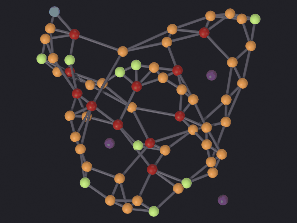
The three purple nodes are the isolated ones: degree 0, sitting in the gaps of a network they are not part of. A force layout has nothing to say about where they belong, because the only thing that would say it is an edge, so they are placed by repulsion alone, wherever there is room. Honest, but in the figure indistinguishable from a genuinely peripheral node, which is the other reason to drop them before the layout.

Other operators in this panel

Two more layout operators sit next to apply_layout, and neither does what its label suggests.

scigraphs.reset_layout returns the graph to random positions, drawn with a bare np.random.rand (SciGraphs/ui/operators/scigraphs/layout_operators.py:478), not through get_geometry_seed() the way the mesh builder does. So “reset” does not return the positions the graph was created with, and two resets do not agree with each other. It also clears the object’s animation data, the part you want after an execute_layout_step run has keyframed sixty frames of positions onto it.

scigraphs.network_splitter_3d moves nodes, but as a post-process: it takes an existing layout and separates it into Z layers by community, degree or an attribute. It belongs with the topology material of notebook 05.

before_reset = positions(graph).copy()
sg.graphs.activate(graph)
with nb.quiet():
    bpy.ops.scigraphs.reset_layout()
after_one = positions(graph).copy()
with nb.quiet():
    bpy.ops.scigraphs.reset_layout()
after_two = positions(graph).copy()

check("reset_layout does not reproduce itself",
      float(np.abs(after_one - after_two).max()) > 1e-6,
      "two resets, two different sets of positions")

Info: Layout reset to random positions
Info: Layout reset to random positions
[PASS] reset_layout does not reproduce itself — two resets, two different sets of positions

True

Rendering

Every figure is EEVEE through nb.figure(), look='ink', top-down and orthographic, colored by node_block for the comparisons and by node_shift, node_late_move or node_degree where the subject is the layout itself. Section 1 covers the ramp and the per-panel node radius; notebook 13 the render path, notebook 16 what turbo costs a reader. The panels hold the graph, attribute, colormap, resolution and camera fixed, and are still not comparable in size.

The Vulkan warning applies here as everywhere: on Blender’s Vulkan backend, the default on Linux, gpu.state.point_size_set is a no-op for the add-on’s shaders, so POINT and DISK nodes come out one pixel wide. Start Blender with --gpu-backend opengl for any render you intend to look at.

Save

out_dir = nb.out("02_layouts")
out_dir.mkdir(parents=True, exist_ok=True)

# `stochastic_block_model` leaves the partition on the graph as a list of sets,
# and GraphML has no type for that.
export = nx.Graph()
export.add_nodes_from((n, {"block": int(block[n])}) for n in G.nodes())
export.add_edges_from(G.edges())
nx.write_graphml(export, out_dir / "sbm_240.graphml")

import csv

with open(out_dir / "layout_comparison.csv", "w", newline="",
          encoding="utf-8") as handle:
    writer = csv.writer(handle)
    writer.writerow(["algorithm", "seconds", "extent_bu", "median_nn_bu",
                    "node_radius_bu", "block_ratio", "hidden_in_plan",
                    "z_share"])
    for algorithm, s in panel_stats.items():
        writer.writerow([algorithm, f"{s['seconds']:.3f}", f"{s['extent']:.4f}",
                        f"{s['median_nn']:.5f}", f"{s['radius']:.5f}",
                        f"{s['ratio']:.4f}", f"{s['hidden']:.4f}",
                        f"{s['z_share']:.4f}"])

with open(out_dir / "layout_timings.csv", "w", newline="",
          encoding="utf-8") as handle:
    writer = csv.writer(handle)
    writer.writerow(["nodes", "algorithm", "seconds"])
    for (n, algorithm), seconds in timings.items():
        writer.writerow([n, algorithm, f"{seconds:.3f}"])

print("written to", nb.rel(out_dir))
for path in sorted(out_dir.iterdir()):
    print("  ", path.name, f"{path.stat().st_size / 1e3:.0f} kB")

written to notebooks/out/02_layouts
   layout_comparison.csv 1 kB
   layout_timings.csv 0 kB
   sbm_240.graphml 47 kB

Summary

Question	Answer, as measured here
Does a layout repeat?	Only FORCEATLAS2 among the force layouts; IGRAPH_KK, SPECTRAL_3D, MDS_3D, GRAPHVIZ_DOT, GRID, SPHERE and RANDOM are deterministic outright
Does the seed matter?	It moves the picture (median residual ≈ 0.5 RMS radii after alignment) and not the finding (block ratio agrees to three decimals)
Does scale mean anything?	Not across algorithms: extent 5.4 to 140 Blender units at the same scale=5.0
What does a plan cost a 3D layout?	27 to 35 % of the nodes hidden behind another, and 0.003 to 0.014 of the structure score. SPHERE is the exception: it improves by 0.14, which is why that score cannot be trusted for it
What scales?	sfdp / YIFAN_HU, IGRAPH_FR, SPECTRAL_3D: sub-second at 3,000 nodes. SPRING_3D and IGRAPH_KK are quadratic
What will crash?	sfdp with default smoothing on a graph containing an isolated node: abort(), status 134, no exception
What will be lost?	Every EDGE-domain attribute, on every layout, silently zeroed. Lay out first, measure the edges second

The rule the notebook argues for: a layout is part of the method, not part of the presentation. Report which algorithm, which parameters and which seed, and quote a measurement over the relations rather than a description of the picture.

Next: 17 · Centrality, which puts a number on each node and needs a layout to show it, so it inherits everything above.