01 · Abstract graphs

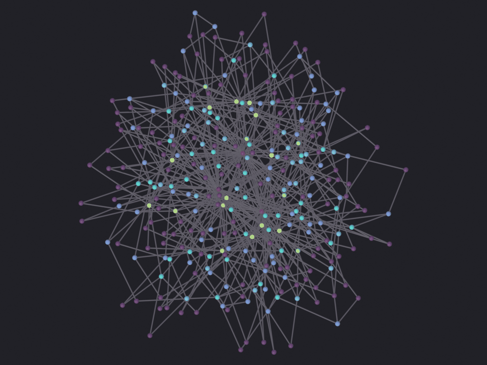
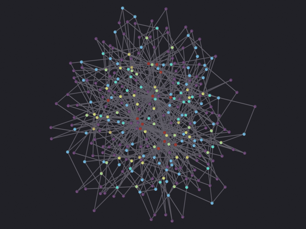
A graph here is combinatorial, with no position until a layout gives it one, which is notebook 02’s subject. Getting one in while keeping its attributes intact is the hard part.

Two innocuous column names, density and max_load, send the importer down its geospatial branch, because it matches latitude and longitude by the bare substrings y and x: it builds a globe and posts the node identifiers to a geocoder. The layout that runs on import zeroes every edge attribute it just read, and an edge list cannot express an isolated node, so one of three hundred quietly fails to arrive.

01 · Abstract graphs (graphs that are not anywhere)

In notebooks 06 to 19 the nodes arrive with coordinates and the drawing is a measurement: two nodes are far apart on the page because they are far apart on the ground. An abstract graph is a set of nodes and a set of pairs, nothing else. Every position below was invented by a layout algorithm, and a different algorithm or seed invents different ones for the same graph. Hence 16 · Layouts.

Here: edge list and adjacency matrix into Blender, and Python values onto the mesh as attributes, the currency 17 · Centrality, 18 · Algorithms and 19 · Topology spend. The graphs are NetworkX generators plus one real sparse matrix from SuiteSparse. No internet needed; section 7 is a switch, off by default.

0 · Setup

import pathlib
import sys


def find_repo():
    """Locate the SciGraphs repository, without relying on the cwd.

    In a normal Jupyter the kernel starts per notebook with the cwd set to its
    folder. Not here: the kernel lives inside Blender and existed before you
    opened anything, so the cwd is wherever Blender was launched from. What the
    extension does know is which folder it is serving to JupyterLab.
    """
    candidates = []
    try:
        import bpy
        prefs = bpy.context.preferences.addons[
            "bl_ext.user_default.jupyter_blender"].preferences
        candidates.append(pathlib.Path(bpy.path.abspath(prefs.notebook_dir)))
    except Exception:
        pass
    candidates.append(pathlib.Path.cwd())

    for base in candidates:
        for directory in (base, *base.parents):
            if (directory / "SciGraphs" / "api" / "graphs.py").is_file():
                return directory

    raise RuntimeError(
        "Cannot find the SciGraphs repository. Point at it by hand:\n"
        "    sys.path.insert(0, '/path/to/SciGraphs-1/notebooks/tools')")


sys.path.insert(0, str(find_repo() / "notebooks" / "tools"))

import bpy
import networkx as nx
import numpy as np
import pandas as pd

# `nb` must import first: it puts this repository on sys.path, so the
# `SciGraphs` import below reads this tree, not the copy Blender installed.
import nb
from nb import check

from SciGraphs import api as sg

# `SEED` goes to the NetworkX generators. `LAYOUT_SEED` goes to NumPy's global
# RNG immediately before each import, which is what the default 2D spring
# layout draws from, not the add-on's own layout RNG (section 2 measures it).
SEED = 42
LAYOUT_SEED = 7

OUT = nb.out("15_abstract")
OUT.mkdir(parents=True, exist_ok=True)

print("networkx", nx.__version__)
print("working directory for this notebook:", nb.rel(OUT))

networkx 3.6
working directory for this notebook: notebooks/out/15_abstract

1 · Four graphs, no coordinates

Chosen for what they disagree about: a figure that works for one can be a lie about another.

Generator	What it models	The property that matters here
karate_club_graph()	a real 1970s social network, 34 people	small enough to read node by node
erdos_renyi_graph(n, p)	pure chance	degrees cluster around the mean
barabasi_albert_graph(n, m)	preferential attachment	degrees are heavy-tailed: a few hubs
watts_strogatz_graph(n, k, p)	a ring with shortcuts	the interesting structure is on the edges

GRAPHS = {
    "karate":  nx.karate_club_graph(),
    "random":  nx.erdos_renyi_graph(300, 0.02, seed=SEED),
    "scale_free": nx.barabasi_albert_graph(300, 2, seed=SEED),
    "small_world": nx.watts_strogatz_graph(240, 6, 0.08, seed=SEED),
}

rows = []
for name, G in GRAPHS.items():
    degrees = np.array([d for _, d in G.degree()], dtype=float)
    rows.append({
                "graph": name,
                "nodes": G.number_of_nodes(),
                "edges": G.number_of_edges(),
                "mean_degree": round(degrees.mean(), 2),
                "max_degree": int(degrees.max()),
                "max/median": round(degrees.max() / max(np.median(degrees), 1.0), 1),
                "components": nx.number_connected_components(G),
                "isolated": len(list(nx.isolates(G))),
                })
print(pd.DataFrame(rows).to_string(index=False))

check("no generator gives its nodes a position",
      all(not any("pos" in d or "x" in d for _, d in G.nodes(data=True))
      for G in GRAPHS.values()),
      "there is nothing in these objects but nodes and pairs")

      graph  nodes  edges  mean_degree  max_degree  max/median  components  isolated
     karate     34     78         4.59          17         5.7           1         0
     random    300    889         5.93          19         3.2           2         1
 scale_free    300    596         3.97          55        18.3           1         0
small_world    240    720         6.00           8         1.3           1         0
[PASS] no generator gives its nodes a position — there is nothing in these objects but nodes and pairs

True

2 · Getting one in: the edge list

bpy.ops.scigraphs.create_graph, behind the Create Graph button, takes no graph argument; it reads the scene’s import settings, which the panel writes into. Same three steps as the GUI, same order:

1. scene.scigraphs.filepath: a CSV (or a .gexf). First, and not for tidiness: source_column and target_column are dynamic enums rebuilt from the header whenever they are touched (SciGraphs/properties/callbacks.py:21). With no filepath the only item is '0', and assigning anything else raises TypeError.
2. bpy.ops.scigraphs.load_columns(): reads the header, guesses a type per column, fills the import as attribute checkboxes section 4 needs, and runs the geospatial auto-detection warned about below.
3. bpy.ops.scigraphs.create_graph().

The column properties hold the column’s index as a string, not its name.

def write_edge_csv(G, path, edge_columns=()):
    """One row per edge: source, target, and one column per callable given.

    `edge_columns` is a sequence of `(name, fn)` where `fn(u, v)` returns a
    number. This is the format `create_graph` expects, and the *only* thing it
    expects: an edge list has no way to say that a node exists. Section 6
    measures what that costs.
    """
    frame = pd.DataFrame(
        [{"source": u, "target": v,
         **{name: fn(u, v) for name, fn in edge_columns}}
         for u, v in G.edges()])
    frame.to_csv(path, index=False)
    return path


def import_edge_list(path, name, auto_layout=True, layout='SPRING',
                     layout_seed=LAYOUT_SEED, directed=False):
    """The three-step operator route, plus the seed the add-on does not set."""
    props = bpy.context.scene.scigraphs
    props.filepath = str(path)                # must precede the two enums
    props.csv_delimiter = ','
    bpy.ops.scigraphs.load_columns()
    props.use_geospatial = False              # see the warning below
    props.source_column = '0'
    props.target_column = '1'
    props.is_directed = directed
    props.remove_self_loops = True
    props.auto_layout_on_import = auto_layout
    props.layout_algorithm = layout
    props.layout_scale = 5.0
    np.random.seed(layout_seed)               # see the note below
    # Read the status, do not rely on an exception. Under `blender -b` an
    # operator error raises `RuntimeError`, but a live session swallows it and
    # returns `{'CANCELLED'}`, so `try`/`except` passes in the harness and
    # silently believes a failed import in front of a reader.
    status = bpy.ops.scigraphs.create_graph()
    if 'FINISHED' not in status:
        raise RuntimeError(f"create_graph returned {set(status)}")
    obj = bpy.context.active_object
    obj.name = name
    return obj


sg.graphs.clear_scene(keep_anchor=False)

karate_csv = write_edge_csv(GRAPHS["karate"], OUT / "karate_edges.csv")
print(pathlib.Path(karate_csv).read_text().splitlines()[:4])

karate = import_edge_list(karate_csv, "Karate")
print()
print(sg.graphs.summary(karate))

['source,target', '0,1', '0,2', '0,3']
Info: Loaded 2 columns
Loading graph from notebooks/out/15_abstract/karate_edges.csv...
  CSV read in 0.00s
  Edges extracted in 0.00s
  Nodes extracted in 0.00s
Total load time: 0.00s
  Nodes: 34, Edges: 78

Creating graph object with 34 nodes...
  Random positions generated in 0.00s (seed=1426602425)
  Vertices created in 0.00s
  78 edges created in 0.00s
  Mesh conversion in 0.00s
  Object created in 0.00s
DataFrame columns: ['source', 'target']
DataFrame shape: (78, 2)
Source column: source, Target column: target
Number of mesh vertices: 34
Number of mesh edges: 78
Selected attributes for import: ['source', 'target']
Imported 0 attribute columns
  Attributes imported in 0.00s
Total graph creation time: 0.00s

======================================================================
Layout algorithm: SPRING
Graph: 34 nodes, 78 edges
Parameters:
  - algorithm: SPRING
  - iterations: 50
  - scale: 5.0000
  - num_nodes: 34
  - num_edges: 78
Execution time: 0.003s
Status: success
======================================================================

Info: Auto-layout applied: SPRING
Info: Graph created: 34 nodes, 78 edges (SPRING layout applied)

{'object': 'Karate', 'type': 'MESH', 'num_nodes': 34, 'num_edges': 78, 'is_directed': False, 'vertices': 34, 'mesh_edges': 78, 'attributes': ['node_id', 'position', '.edge_verts', '.corner_vert', '.corner_edge']}

Both the topology and the identifiers have failed to survive this trip silently before.

def node_names(obj):
    """The graph's node identifiers, in mesh-vertex order.

    SciGraphs stores them as one comma-joined string in a custom property
    (`SciGraphs/core/mesh/geometry.py:383`), so vertex *i* is `names[i]` and
    that is the only way back from a mesh index to a name.
    """
    return obj.get("nodes_data", "").split(",")


def edge_pairs(obj):
    """The (i, j) vertex indices of every mesh edge, in mesh-edge order."""
    flat = np.empty(len(obj.data.edges) * 2, dtype=np.int32)
    obj.data.edges.foreach_get("vertices", flat)
    return flat.reshape(-1, 2)


names = node_names(karate)
imported = {frozenset((int(names[a]), int(names[b]))) for a, b in edge_pairs(karate)}
original = {frozenset(e) for e in GRAPHS["karate"].edges()}

check("every node arrived", len(names) == GRAPHS["karate"].number_of_nodes(),
      f"{len(names)} names, first four {names[:4]}")
check("the edge set is identical", imported == original,
      f"{len(imported)} mesh edges vs {len(original)} in NetworkX")

[PASS] every node arrived — 34 names, first four ['0', '1', '2', '3']
[PASS] the edge set is identical — 78 mesh edges vs 78 in NetworkX

True

Defect: load_columns can turn an abstract import into a geospatial one from the column names alone. Its last act, scigraphs.detect_geospatial (data_operators.py:127), matches latitude and longitude columns by substring against ['lat', 'latitude', 'y', 'coord_y'] and ['lon', 'long', 'longitude', 'x', 'coord_x'] (SciGraphs/core/geo/geospatial.py:40). A bare 'y' matches any numeric column containing the letter y (density, entropy, community, delay); 'x' matches max_load, index, flux. Both hitting sets props.use_geospatial to True for good, and the next create_graph takes the geospatial branch (data_operators.py:212): a globe, and with geocode_columns defaulting to True (properties/scene_properties.py:215), the identifiers go through Nominatim as place names. That is a network call, so the cell below stops at the detection. Fix: use_geospatial = False after load_columns, as import_edge_list does.

trap_csv = OUT / "innocent_column_names.csv"
pd.DataFrame([{"source": u, "target": v, "density": 0.5, "max_load": 2.0}
             for u, v in list(GRAPHS["karate"].edges())[:10]]).to_csv(
             trap_csv, index=False)

props = bpy.context.scene.scigraphs
props.use_geospatial = False
props.filepath = str(trap_csv)
bpy.ops.scigraphs.load_columns()

print(f"columns          : {[i.name for i in props.available_csv_columns]}")
print(f"use_geospatial   : {props.use_geospatial}")
print(f"latitude column  : {props.latitude_column}  "
      f"longitude column: {props.longitude_column}")

check("two ordinary column names switched the importer to globe mode",
      props.use_geospatial,
      "'density' matched the 'y' pattern, 'max_load' matched 'x'")
props.use_geospatial = False

Detected geospatial columns: density, max_load
Info: Detected geospatial columns: density, max_load
Info: Loaded 4 columns
columns          : ['source', 'target', 'density', 'max_load']
use_geospatial   : True
latitude column  : 2  longitude column: 3
[PASS] two ordinary column names switched the importer to globe mode — 'density' matched the 'y' pattern, 'max_load' matched 'x'

Defect: node identifiers are a comma-joined string. nodes_data and edges_data are built with ",".join(...) (SciGraphs/core/mesh/geometry.py:383 and :394) and split back with str.split(",") (SciGraphs/core/mesh/layouts/common.py:118, :126). A node whose name contains a comma shifts every identifier after it. Not for long: the layout raises IndexError at common.py:126, several steps from the cause. Integers or bare words are safe; spreadsheet output is not.

comma_csv = OUT / "comma_labels.csv"
pd.DataFrame({"source": ["Smith, J.", "Lee"], "target": ["Lee", "Ng"]}).to_csv(
    comma_csv, index=False)

before = set(bpy.data.objects)

# Layout off, or it reads the identifiers back and dies with `IndexError` from
# `layouts/common.py:126`. That crash is not catchable here: `bpy.ops` hands it
# to `sys.excepthook` and returns `{'CANCELLED'}`, and in a live kernel that
# hook is IPython's, which fails the cell while the surrounding `try` sees
# nothing. Off, the damage can be inspected instead.
comma_obj = import_edge_list(comma_csv, "CommaLabels", auto_layout=False)

print("nodes_data:", comma_obj["nodes_data"])
print("edges_data:", comma_obj["edges_data"])

# A comma in a name becomes two identifiers, so the edge reader, pairing tokens
# two at a time, runs off the end.
tokens = comma_obj["edges_data"].split(",")
print(f"\n{len(tokens)} tokens for {comma_obj['num_edges']} edges, "
      f"{2 * comma_obj['num_edges']} expected")
check("a comma in a node name corrupts the stored identifiers",
      len(tokens) != 2 * comma_obj["num_edges"],
      "quote it out of the CSV, or rename before import; with the "
      "automatic layout on, this same string aborts the import")

for obj in set(bpy.data.objects) - before:
    bpy.data.objects.remove(obj, do_unlink=True)

Info: Loaded 2 columns
Loading graph from notebooks/out/15_abstract/comma_labels.csv...
  CSV read in 0.00s
  Edges extracted in 0.00s
  Nodes extracted in 0.00s
Total load time: 0.00s
  Nodes: 3, Edges: 2

Creating graph object with 3 nodes...
  Random positions generated in 0.00s (seed=1426602425)
  Vertices created in 0.00s
  2 edges created in 0.00s
  Mesh conversion in 0.00s
  Object created in 0.00s
DataFrame columns: ['source', 'target']
DataFrame shape: (2, 2)
Source column: source, Target column: target
Number of mesh vertices: 3
Number of mesh edges: 2
Imported 0 attribute columns
  Attributes imported in 0.00s
Total graph creation time: 0.00s
Info: Graph created: 3 nodes, 2 edges
nodes_data: Lee,Ng,Smith, J.
edges_data: Smith, J.,Lee,Lee,Ng

5 tokens for 2 edges, 4 expected
[PASS] a comma in a node name corrupts the stored identifiers — quote it out of the CSV, or rename before import; with the automatic layout on, this same string aborts the import

The layout is not part of the graph

With auto_layout_on_import on, the default, create_graph also ran a layout and wrote the result into node_positions.

Defect: the default 2D spring layout is not reproducible. _spring_layout_2d calls nx.spring_layout(...) with no seed= (SciGraphs/core/mesh/layouts/networkx_layouts.py:8, 3D twin at :18), so it draws from NumPy’s global RNG. The module keeps a seeded generator for exactly this, _reset_layout_rng() at the top of every apply_graph_layout (SciGraphs/core/mesh/layouts/dispatcher.py:22), and then does not pass it in. Two imports of one file give two different drawings. Seeding np.random immediately before the operator, as import_edge_list does, is the workaround; FORCEATLAS2 threads the seeded generator through (layouts/forceatlas.py:41) and does not need it.

def positions(obj):
    return np.asarray(list(obj["node_positions"]), dtype=float).reshape(-1, 3)


unseeded_a = import_edge_list(karate_csv, "Unseeded_A", layout_seed=None)
unseeded_b = import_edge_list(karate_csv, "Unseeded_B", layout_seed=None)
seeded_a = import_edge_list(karate_csv, "Seeded_A", layout_seed=11)
seeded_b = import_edge_list(karate_csv, "Seeded_B", layout_seed=11)

drift = np.abs(positions(unseeded_a) - positions(unseeded_b)).max()
print(f"unseeded, two runs: largest disagreement {drift:.3f} Blender units "
      f"(the drawing is ~10 across)")
print(f"seeded, two runs  : largest disagreement "
      f"{np.abs(positions(seeded_a) - positions(seeded_b)).max():.3f}")

check("the unseeded layout is not reproducible", drift > 0.1)
check("seeding numpy first makes it reproducible",
      np.allclose(positions(seeded_a), positions(seeded_b)))
check("the topology never depended on the seed",
      {frozenset((int(node_names(seeded_a)[a]), int(node_names(seeded_a)[b])))
      for a, b in edge_pairs(seeded_a)} == original,
      "different pictures, same graph")

for obj in (unseeded_a, unseeded_b, seeded_a, seeded_b):
    bpy.data.objects.remove(obj, do_unlink=True)

Info: Loaded 2 columns
Loading graph from notebooks/out/15_abstract/karate_edges.csv...
  CSV read in 0.00s
  Edges extracted in 0.00s
  Nodes extracted in 0.00s
Total load time: 0.00s
  Nodes: 34, Edges: 78

Creating graph object with 34 nodes...
  Random positions generated in 0.00s (seed=1426602425)
  Vertices created in 0.00s
  78 edges created in 0.00s
  Mesh conversion in 0.00s
  Object created in 0.00s
DataFrame columns: ['source', 'target']
DataFrame shape: (78, 2)
Source column: source, Target column: target
Number of mesh vertices: 34
Number of mesh edges: 78
Selected attributes for import: ['source', 'target']
Imported 0 attribute columns
  Attributes imported in 0.00s
Total graph creation time: 0.00s

======================================================================
Layout algorithm: SPRING
Graph: 34 nodes, 78 edges
Parameters:
  - algorithm: SPRING
  - iterations: 50
  - scale: 5.0000
  - num_nodes: 34
  - num_edges: 78
Execution time: 0.003s
Status: success
======================================================================

Info: Auto-layout applied: SPRING
Info: Graph created: 34 nodes, 78 edges (SPRING layout applied)
Info: Loaded 2 columns
Loading graph from notebooks/out/15_abstract/karate_edges.csv...
  CSV read in 0.00s
  Edges extracted in 0.00s
  Nodes extracted in 0.00s
Total load time: 0.00s
  Nodes: 34, Edges: 78

Creating graph object with 34 nodes...
  Random positions generated in 0.00s (seed=1426602425)
  Vertices created in 0.00s
  78 edges created in 0.00s
  Mesh conversion in 0.00s
  Object created in 0.00s
DataFrame columns: ['source', 'target']
DataFrame shape: (78, 2)
Source column: source, Target column: target
Number of mesh vertices: 34
Number of mesh edges: 78
Selected attributes for import: ['source', 'target']
Imported 0 attribute columns
  Attributes imported in 0.00s
Total graph creation time: 0.00s

======================================================================
Layout algorithm: SPRING
Graph: 34 nodes, 78 edges
Parameters:
  - algorithm: SPRING
  - iterations: 50
  - scale: 5.0000
  - num_nodes: 34
  - num_edges: 78
Execution time: 0.003s
Status: success
======================================================================

Info: Auto-layout applied: SPRING
Info: Graph created: 34 nodes, 78 edges (SPRING layout applied)
Info: Loaded 2 columns
Loading graph from notebooks/out/15_abstract/karate_edges.csv...
  CSV read in 0.00s
  Edges extracted in 0.00s
  Nodes extracted in 0.00s
Total load time: 0.00s
  Nodes: 34, Edges: 78

Creating graph object with 34 nodes...
  Random positions generated in 0.00s (seed=1426602425)
  Vertices created in 0.00s
  78 edges created in 0.00s
  Mesh conversion in 0.00s
  Object created in 0.00s
DataFrame columns: ['source', 'target']
DataFrame shape: (78, 2)
Source column: source, Target column: target
Number of mesh vertices: 34
Number of mesh edges: 78
Selected attributes for import: ['source', 'target']
Imported 0 attribute columns
  Attributes imported in 0.00s
Total graph creation time: 0.00s

======================================================================
Layout algorithm: SPRING
Graph: 34 nodes, 78 edges
Parameters:
  - algorithm: SPRING
  - iterations: 50
  - scale: 5.0000
  - num_nodes: 34
  - num_edges: 78
Execution time: 0.003s
Status: success
======================================================================

Info: Auto-layout applied: SPRING
Info: Graph created: 34 nodes, 78 edges (SPRING layout applied)
Info: Loaded 2 columns
Loading graph from notebooks/out/15_abstract/karate_edges.csv...
  CSV read in 0.00s
  Edges extracted in 0.00s
  Nodes extracted in 0.00s
Total load time: 0.00s
  Nodes: 34, Edges: 78

Creating graph object with 34 nodes...
  Random positions generated in 0.00s (seed=1426602425)
  Vertices created in 0.00s
  78 edges created in 0.00s
  Mesh conversion in 0.00s
  Object created in 0.00s
DataFrame columns: ['source', 'target']
DataFrame shape: (78, 2)
Source column: source, Target column: target
Number of mesh vertices: 34
Number of mesh edges: 78
Selected attributes for import: ['source', 'target']
Imported 0 attribute columns
  Attributes imported in 0.00s
Total graph creation time: 0.00s

======================================================================
Layout algorithm: SPRING
Graph: 34 nodes, 78 edges
Parameters:
  - algorithm: SPRING
  - iterations: 50
  - scale: 5.0000
  - num_nodes: 34
  - num_edges: 78
Execution time: 0.003s
Status: success
======================================================================

Info: Auto-layout applied: SPRING
Info: Graph created: 34 nodes, 78 edges (SPRING layout applied)
unseeded, two runs: largest disagreement 6.024 Blender units (the drawing is ~10 across)
seeded, two runs  : largest disagreement 0.000
[PASS] the unseeded layout is not reproducible
[PASS] seeding numpy first makes it reproducible
[PASS] the topology never depended on the seed — different pictures, same graph

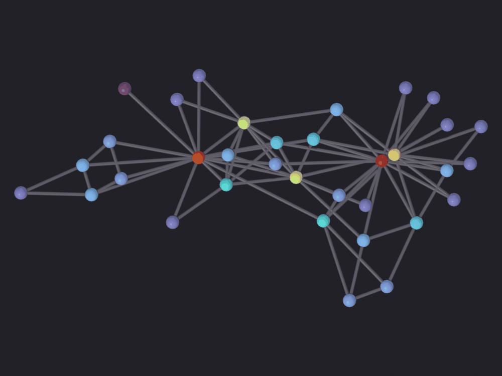
The first figure

Every figure here is an EEVEE render straight down through an orthographic camera (nb.figure’s default) with look='ink': turbo colormap, the darkest of the five backdrops. Thin lines and small glyphs on empty space need a ramp that never passes near the backdrop, and turbo runs from dark blue to red, the same reason 03 uses it. The ramp always carries a quantity the notebook computed, here node degree. The camera assumes the drawing is flat; SPRING is planar, and section 5 measures what the three-dimensional default would cost.

def set_point_attribute(obj, name, values):
    """Write a per-node float onto the mesh as a POINT attribute.

    `values` is indexed the same way as `node_names(obj)`, in vertex order.
    """
    mesh = obj.data
    if name in mesh.attributes:
        mesh.attributes.remove(mesh.attributes[name])
    attr = mesh.attributes.new(name=name, type='FLOAT', domain='POINT')
    attr.data.foreach_set("value", np.asarray(values, dtype=np.float32).tolist())
    return name


degree = {n: float(d) for n, d in GRAPHS["karate"].degree()}
set_point_attribute(karate, "degree",
                    [degree[int(n)] for n in node_names(karate)])

print("attributes on the karate graph:")
for name, domain, dtype in sg.graphs.attributes(karate):
    print(f"  {name:<28} {domain:<7} {dtype}")

check("degree arrived as a POINT attribute",
      sg.render.attribute_domain(karate, "degree") == 'POINT')

attributes on the karate graph:
  node_id                      POINT   INT
  position                     POINT   FLOAT_VECTOR
  .edge_verts                  EDGE    INT32_2D
  .corner_vert                 CORNER  INT
  .corner_edge                 CORNER  INT
  degree                       POINT   FLOAT
[PASS] degree arrived as a POINT attribute

True

Node size is not left alone. render_eevee derives the glyph radius from the graph, the median nearest-neighbor distance times node_fraction; a radius chosen in the abstract has produced both 97.8 %-ink mats and invisible specks here. The default 0.35 was calibrated on a street network, where intersection spacing is irregular. A force layout equalizes spacing, so the median is a tighter bound and 0.35 spends it on the glyphs.

for fraction in (0.35, 0.22):
    path = nb.render(
        karate, f"renders/01_abstract/1_karate_nf{fraction}",
        look='ink', color_attribute="degree",
        node_fraction=fraction, verbose=False)
    print(f"node_fraction {fraction}: radius "
          f"{karate['scigraphs_node_size']:.4f} BU, ink {nb.ink(path) * 100:.1f} %")
    nb.check_render(path)

nb.show(nb.out("renders/01_abstract/1_karate_nf0.22.png"))

Info: Geometry Nodes modifier added
Info: Attribute -> degree  ·  degree -> turbo  [1 … 17] on Point
node_fraction 0.35: radius 0.1962 BU, ink 14.6 %
[PASS] 1_karate_nf0.35.png legible — 14.6% ink (healthy range 0.5–60%)
Info: Geometry Nodes modifier added
Info: Attribute -> degree  ·  degree -> turbo  [1 … 17] on Point
node_fraction 0.22: radius 0.1233 BU, ink 10.0 %
[PASS] 1_karate_nf0.22.png legible — 10.0% ink (healthy range 0.5–60%)

True

3 · The other format: an adjacency matrix

Notebook 15 had od_matrix_to_graph() accept an edge list or a square matrix. The abstract importer does not: create_graph reads a CSV of rows and load_graph_from_file (SciGraphs/core/data_io/importer.py:105) takes two column indices out of it. There is no matrix_type on this path, and a square matrix would be read as an edge list between its first two columns. Converting by hand rather than with nx.from_numpy_array keeps the mapping from row index back to node identifier in view.

small_world = GRAPHS["small_world"]
labels = sorted(small_world.nodes())
A = nx.to_numpy_array(small_world, nodelist=labels)

upper_i, upper_j = np.triu_indices_from(A, k=1)
nonzero = A[upper_i, upper_j] > 0
matrix_edges = pd.DataFrame({
                            "source": [labels[i] for i in upper_i[nonzero]],
                            "target": [labels[j] for j in upper_j[nonzero]],
})
matrix_csv = OUT / "small_world_from_matrix.csv"
matrix_edges.to_csv(matrix_csv, index=False)

print(f"matrix {A.shape}, {int(A.sum() / 2)} undirected non-zero cells")
print(f"edge list written from it: {len(matrix_edges)} rows")

check("the matrix and the edge list describe the same graph",
      {frozenset(e) for e in matrix_edges.itertuples(index=False, name=None)}
      == {frozenset(e) for e in small_world.edges()},
      "the round trip through a dense matrix is lossless for an "
      "unweighted, undirected graph")

matrix (240, 240), 720 undirected non-zero cells
edge list written from it: 720 rows
[PASS] the matrix and the edge list describe the same graph — the round trip through a dense matrix is lossless for an unweighted, undirected graph

True

Two asymmetries, and why the edge list is the native format:

• A dense matrix costs n² whatever the graph is. The small-world graph is 240 × 240 = 57,600 cells for 720 edges, 1.2 % occupancy. At 10,000 nodes it is 800 MB against a few megabytes of edge list.
• The matrix can say something the edge list cannot: a row and column of zeros is an isolated node. Section 6 is where that matters.

density = small_world.number_of_edges() / (A.shape[0] * (A.shape[0] - 1) / 2)
print(f"occupancy of the dense matrix: {density * 100:.2f} %")
print(f"dense at 10,000 nodes        : {10_000 ** 2 * 8 / 1e6:.0f} MB of float64")

occupancy of the dense matrix: 2.51 %
dense at 10,000 nodes        : 800 MB of float64

4 · Attributes are the currency

Everything downstream reads mesh attributes: figure color, sizes in a Geometry Nodes tree, layout weighting, every measure notebooks 03 to 05 compute. So the question about an import route is whether the numbers survive. Three routes, none alike.

Route 1: extra columns in the edge CSV. Any numeric column that is not source or target is imported twice: onto the edges as edge_<column>, and onto the nodes as five aggregates, vertex_<column>_{sum,mean,min,max,count} (SciGraphs/core/mesh/geometry.py:513 and :537). The prefix is vertex_, not the node_ the geospatial importer uses, so notebooks 17 to 19 cannot assume one convention.

The small-world graph’s interesting quantity is an edge property: how far apart two nodes are on the original ring. A lattice edge joins near neighbors, a rewired shortcut joins the far side.

N_RING = small_world.number_of_nodes()


def ring_gap(u, v):
    """Distance between two node indices around the ring they started on."""
    d = abs(int(u) - int(v))
    return min(d, N_RING - d)


sw_csv = write_edge_csv(small_world, OUT / "small_world_edges.csv",
                        edge_columns=[("ring_gap", ring_gap)])
print(pathlib.Path(sw_csv).read_text().splitlines()[:4])

sw = import_edge_list(sw_csv, "SmallWorld")

print()
print("attributes after import:")
for name, domain, dtype in sg.graphs.attributes(sw):
    if not name.startswith("."):
        print(f"  {name:<28} {domain:<7} {dtype}")

['source,target,ring_gap', '0,1,1', '0,239,1', '0,238,2']
Info: Loaded 3 columns
Loading graph from notebooks/out/15_abstract/small_world_edges.csv...
  CSV read in 0.00s
  Edges extracted in 0.00s
  Nodes extracted in 0.00s
Total load time: 0.00s
  Nodes: 240, Edges: 720

Creating graph object with 240 nodes...
  Random positions generated in 0.00s (seed=1426602425)
  Vertices created in 0.00s
  720 edges created in 0.00s
  Mesh conversion in 0.00s
  Object created in 0.00s
DataFrame columns: ['source', 'target', 'ring_gap']
DataFrame shape: (720, 3)
Source column: source, Target column: target
Number of mesh vertices: 240
Number of mesh edges: 720
Selected attributes for import: ['source', 'target', 'ring_gap']
Processing column 'ring_gap': int64
  Created edge attribute 'edge_ring_gap'
  Created vertex attributes for 'ring_gap': sum, mean, min, max, count
Imported 1 attribute columns
  Attributes imported in 0.01s
Total graph creation time: 0.01s

======================================================================
Layout algorithm: SPRING
Graph: 240 nodes, 720 edges
Parameters:
  - algorithm: SPRING
  - iterations: 50
  - scale: 5.0000
  - num_nodes: 240
  - num_edges: 720
Execution time: 0.065s
Status: success
======================================================================

Info: Auto-layout applied: SPRING
Info: Graph created: 240 nodes, 720 edges (SPRING layout applied)

attributes after import:
  vertex_ring_gap_sum          POINT   FLOAT
  vertex_ring_gap_mean         POINT   FLOAT
  vertex_ring_gap_min          POINT   FLOAT
  vertex_ring_gap_max          POINT   FLOAT
  vertex_ring_gap_count        POINT   INT
  node_id                      POINT   INT
  edge_ring_gap                EDGE    FLOAT
  position                     POINT   FLOAT_VECTOR

Defect: the auto-layout wipes every EDGE attribute. rebuild_edges() restores the mesh’s edges after a layout has moved the vertices by deleting every bmesh edge and creating it again (SciGraphs/core/mesh/geometry.py:1227 to :1248). EDGE-domain custom attributes come back allocated and zeroed. The import operator calls it on every import that applies a layout, the default (SciGraphs/ui/operators/scigraphs/data_operators.py:41), as does every one of the seven layout operators (SciGraphs/ui/operators/scigraphs/layout_operators.py:322, :397, :483, :589, :639). The give-away: the same column survives on the other domain, since rebuild_edges leaves vertices alone, so the vertex_ring_gap_* aggregates are intact. An edge-valued figure comes out uniformly colored and nothing raises.

def read_attribute(obj, name):
    attr = obj.data.attributes[name]
    count = len(obj.data.edges) if attr.domain == 'EDGE' else len(obj.data.vertices)
    values = np.empty(count, dtype=np.float64)
    attr.data.foreach_get("value", values)
    return values


from_operator = read_attribute(sw, "edge_ring_gap")
aggregate = read_attribute(sw, "vertex_ring_gap_max")

print(f"edge_ring_gap        min {from_operator.min():g}  max {from_operator.max():g}")
print(f"vertex_ring_gap_max  min {aggregate.min():g}  max {aggregate.max():g}")

check("the EDGE attribute was zeroed by the layout",
      np.all(from_operator == 0),
      "same CSV column, same import, different domain")
check("the POINT aggregates of the same column survived",
      aggregate.max() > 0)

edge_ring_gap        min 0  max 0
vertex_ring_gap_max  min 3  max 119
[PASS] the EDGE attribute was zeroed by the layout — same CSV column, same import, different domain
[PASS] the POINT aggregates of the same column survived

True

Route 2: write the attribute yourself, after the layout. The general answer to “I computed something in Python and want to see it”. The care goes into the join from mesh index back to node identifier, through nodes_data. Keying on the identifier pair rather than on edge order means the result does not depend on the importer preserving the CSV’s ordering, which it happens to do, but nothing says so.

def set_edge_attribute(obj, name, values_by_pair):
    """Write a per-edge float, keyed by the unordered pair of node identifiers."""
    names = node_names(obj)
    pairs = edge_pairs(obj)
    values = np.zeros(len(pairs), dtype=np.float32)
    unmatched = 0
    for index, (a, b) in enumerate(pairs):
        key = (names[a], names[b])
        if key in values_by_pair:
            values[index] = values_by_pair[key]
        elif (key[1], key[0]) in values_by_pair:
            values[index] = values_by_pair[(key[1], key[0])]
        else:
            unmatched += 1
    mesh = obj.data
    if name in mesh.attributes:
        mesh.attributes.remove(mesh.attributes[name])
    attr = mesh.attributes.new(name=name, type='FLOAT', domain='EDGE')
    attr.data.foreach_set("value", values.tolist())
    return values, unmatched


gaps, unmatched = set_edge_attribute(
    sw, "edge_ring_gap",
    {(str(u), str(v)): float(ring_gap(u, v)) for u, v in small_world.edges()})

print(f"rewritten: {len(gaps)} edges, {unmatched} unmatched, "
      f"range {gaps.min():g} to {gaps.max():g}")
print(f"shortcuts (gap > {small_world.degree(0) // 2}): "
      f"{int((gaps > small_world.degree(0) // 2).sum())}")

check("every mesh edge found its pair in the graph", unmatched == 0)
check("the edge attribute now carries the measurement", gaps.max() > 0)

rewritten: 720 edges, 0 unmatched, range 1 to 119
shortcuts (gap > 3): 52
[PASS] every mesh edge found its pair in the graph
[PASS] the edge attribute now carries the measurement

True

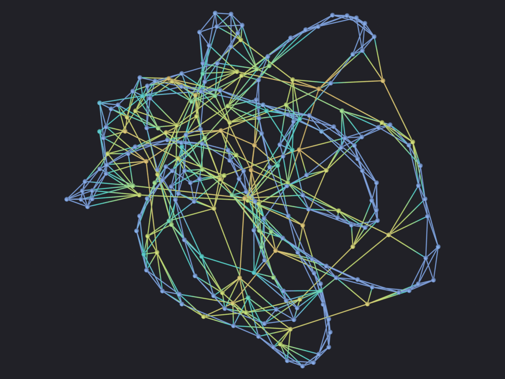
The color scale for a bimodal quantity. ring_gap is not skewed, it is bimodal: lattice edges at 1 to 3, rewired ones scattered up to half the ring. A linear ramp gives 90 % of the edges the bottom 2 % of the scale, and no percentile clip fixes it: clipping moves the top of the ramp and the problem is at the bottom. color_norm='LOG' separates two clusters an order of magnitude apart.

(vmin=/vmax= are silently ineffective: scigraphs.color_set_attribute calls update_property_range() before applying anything (SciGraphs/ui/coloring/operators.py:374) and overwrites both. clip_low_pct/clip_high_pct work.)

linear_share = (np.percentile(gaps, 90) - gaps.min()) / (gaps.max() - gaps.min())
log_share = (np.log(np.percentile(gaps, 90)) - np.log(gaps.min())) / (
    np.log(gaps.max()) - np.log(gaps.min()))
print(f"90 % of the edges fall inside the bottom "
      f"{linear_share * 100:.0f} % of a linear ramp, "
      f"{log_share * 100:.0f} % of a logarithmic one")

90 % of the edges fall inside the bottom 2 % of a linear ramp, 23 % of a logarithmic one

The nodes are deliberately small: the measurement is on the edges, and a glyph large enough to be pleasant hides the data. color_graph leaves the node spheres on the same ramp, where they show the average gap of the edges meeting there.

nb.figure(sw, "renders/01_abstract/2_small_world_ring_gap",
          look='ink', color_attribute="edge_ring_gap",
          color_norm='LOG', node_fraction=0.22)

  Promoted 1 edge attribute(s) to point domain for GN propagation
Info: Geometry Nodes modifier added
Info: Attribute -> edge_ring_gap  ·  edge_ring_gap -> turbo [log]  [1 … 119] on Point

[PASS] 2_small_world_ring_gap.png legible — 15.9% ink (healthy range 0.5–60%)

Route 3: the import_node_attributes operator. The GUI route for per-node values computed elsewhere: identifier in the first column, one value column per attribute. Unlike route 1 it runs after the graph exists, so nothing rebuilds the mesh underneath it; unlike route 2 it is on the panel. Third naming convention on this page: with a header row the attribute takes the column’s name verbatim, no prefix.

karate_graph = GRAPHS["karate"]
attribute_file = OUT / "karate_node_attributes.tsv"
pd.DataFrame({
             "node": list(karate_graph.nodes()),
             "betweenness": [round(v, 6) for v in
             nx.betweenness_centrality(karate_graph).values()],
             "clustering": [round(v, 6) for v in nx.clustering(karate_graph).values()],
}).to_csv(attribute_file, sep="\t", index=False)

props = bpy.context.scene.scigraphs
props.node_attr_filepath = str(attribute_file)
props.node_attr_delimiter = "\t"
props.node_attr_has_header = True

sg.graphs.activate(karate)
print("import_node_attributes ->", bpy.ops.scigraphs.import_node_attributes())
print("names on the mesh now:",
      [n for n, _, _ in sg.graphs.attributes(karate) if not n.startswith(".")])

betweenness = read_attribute(karate, "betweenness")
expected = np.array([nx.betweenness_centrality(karate_graph)[int(n)]
                    for n in node_names(karate)])
check("the values landed on the right vertices",
      np.allclose(betweenness, expected, atol=1e-5),
      f"max disagreement {np.abs(betweenness - expected).max():.2e}")

  Created POINT attribute 'betweenness' (34 nodes matched)
  Created POINT attribute 'clustering' (34 nodes matched)
Imported 2 node attribute(s), 34 nodes matched out of 34
  Rebuilt simple GN tree (attribute stripping updated)
Info: Imported 2 attribute(s): 34/34 nodes matched
import_node_attributes -> {'FINISHED'}
names on the mesh now: ['node_id', 'position', 'degree', 'degree_color', 'betweenness', 'clustering']
[PASS] the values landed on the right vertices — max disagreement 4.88e-07

True

Worth knowing: a node in the graph but absent from the file is given float('nan'), deliberately, so missing data is distinguishable from zero (SciGraphs/core/mesh/geometry.py:658). The coloring pipeline ignores non-finite samples, so a partial file does not distort the ramp, but the nodes it missed take the fallback color and nothing says how many except the operator’s own report. Check the count.

missing = int(np.isnan(betweenness).sum())
print(f"nodes with no value: {missing} of {len(betweenness)}")
check("every node matched a row", missing == 0)

nodes with no value: 0 of 34
[PASS] every node matched a row

True

5 · What is different without coordinates

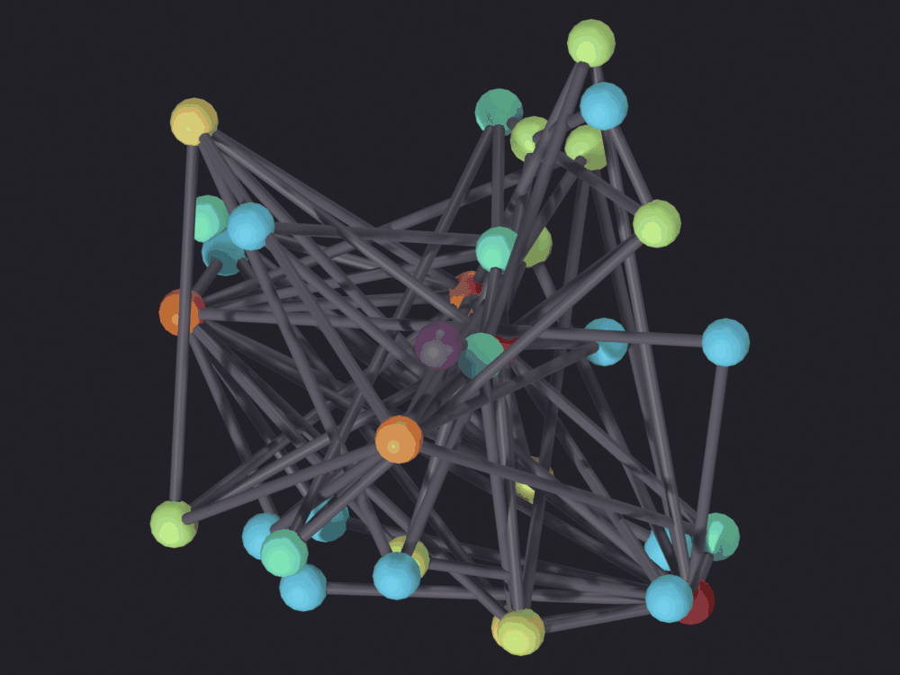
With auto_layout_on_import off, create_graph still produces a valid SciGraphs object, right node count, right edge count, every attribute in place, and puts every vertex at a seeded random point in a 5-unit cube (SciGraphs/core/mesh/geometry.py:297). Same karate graph as figure 1.

raw = import_edge_list(karate_csv, "Karate_NoLayout", auto_layout=False)
set_point_attribute(raw, "degree", [degree[int(n)] for n in node_names(raw)])

extent = positions(raw).max(axis=0) - positions(raw).min(axis=0)
print(f"positions span {extent.round(2)} Blender units: a cube, not a drawing")
check("the topology is identical to figure 1",
      {frozenset((int(node_names(raw)[a]), int(node_names(raw)[b])))
      for a, b in edge_pairs(raw)} == original)

nb.figure(raw, "renders/01_abstract/3_karate_no_layout",
          look='ink', color_attribute="degree", node_fraction=0.22)

Info: Loaded 2 columns
Loading graph from notebooks/out/15_abstract/karate_edges.csv...
  CSV read in 0.00s
  Edges extracted in 0.00s
  Nodes extracted in 0.00s
Total load time: 0.00s
  Nodes: 34, Edges: 78

Creating graph object with 34 nodes...
  Random positions generated in 0.00s (seed=1426602425)
  Vertices created in 0.00s
  78 edges created in 0.00s
  Mesh conversion in 0.00s
  Object created in 0.00s
DataFrame columns: ['source', 'target']
DataFrame shape: (78, 2)
Source column: source, Target column: target
Number of mesh vertices: 34
Number of mesh edges: 78
Selected attributes for import: ['source', 'target']
Imported 0 attribute columns
  Attributes imported in 0.00s
Total graph creation time: 0.00s
Info: Graph created: 34 nodes, 78 edges
positions span [4.66 4.98 4.72] Blender units: a cube, not a drawing
[PASS] the topology is identical to figure 1
Info: Geometry Nodes modifier added
Info: Attribute -> degree  ·  degree -> turbo [log]  [1 … 17] on Point

[PASS] 3_karate_no_layout.png legible — 29.8% ink (healthy range 0.5–60%)

The two figures are the same object in every sense a graph theorist would recognize, and only one can be read. That gap is the subject of 16 · Layouts: which algorithm, in how many dimensions, with what seed, and what the distances are allowed to mean, a question the geospatial notebooks never have to ask. They mean nothing here; the only honest reading of a force layout is topological: this group is more densely wired to itself than to the rest.

The default FORCEATLAS2 is genuinely three-dimensional and the overhead camera throws one axis away, which on the karate graph is not a rounding error. Hence the planar SPRING, the one under which the picture and the computation agree.

flat = import_edge_list(karate_csv, "Karate_FA2", layout='FORCEATLAS2')
span = positions(flat).max(axis=0) - positions(flat).min(axis=0)
print(f"FORCEATLAS2 span x={span[0]:.2f} y={span[1]:.2f} z={span[2]:.2f}")
print(f"the axis the camera discards is {span[2] / max(span[0], span[1]) * 100:.0f} % "
      f"of the longest one it keeps")

span_spring = positions(karate).max(axis=0) - positions(karate).min(axis=0)
check("the layout used for these figures is planar", span_spring[2] == 0.0,
      f"SPRING span z={span_spring[2]:.3f}")

bpy.data.objects.remove(flat, do_unlink=True)
raw.hide_render = True

Info: Loaded 2 columns
Loading graph from notebooks/out/15_abstract/karate_edges.csv...
  CSV read in 0.00s
  Edges extracted in 0.00s
  Nodes extracted in 0.00s
Total load time: 0.00s
  Nodes: 34, Edges: 78

Creating graph object with 34 nodes...
  Random positions generated in 0.00s (seed=1426602425)
  Vertices created in 0.00s
  78 edges created in 0.00s
  Mesh conversion in 0.00s
  Object created in 0.00s
DataFrame columns: ['source', 'target']
DataFrame shape: (78, 2)
Source column: source, Target column: target
Number of mesh vertices: 34
Number of mesh edges: 78
Selected attributes for import: ['source', 'target']
Imported 0 attribute columns
  Attributes imported in 0.00s
Total graph creation time: 0.00s
Computing ForceAtlas2 (3D, networkx) for 34 nodes...
  ForceAtlas2 completed in 0.01s

======================================================================
Layout algorithm: FORCEATLAS2
Fallback: using SPRING (2D fallback) instead
   Reason: FORCEATLAS2 library not available
Graph: 34 nodes, 78 edges
Parameters:
  - algorithm: FORCEATLAS2
  - iterations: 50
  - scale: 5.0000
  - num_nodes: 34
  - num_edges: 78
Execution time: 0.006s
Status: success (with fallback)
======================================================================

Info: Auto-layout applied: FORCEATLAS2
Info: Graph created: 34 nodes, 78 edges (FORCEATLAS2 layout applied)
FORCEATLAS2 span x=9.83 y=6.87 z=5.88
the axis the camera discards is 60 % of the longest one it keeps
[PASS] the layout used for these figures is planar — SPRING span z=0.000

6 · Two degree distributions, and one color scale that lies

The Erdős-Rényi and Barabási-Albert graphs have almost the same size and density, and completely different degree distributions. That difference is invisible in the topology checks and decides how a figure has to be colored.

summary = []
for name in ("random", "scale_free"):
    d = np.array([v for _, v in GRAPHS[name].degree()], dtype=float)
    summary.append({"graph": name, "n": len(d), "median": np.median(d),
                   "p98": round(float(np.percentile(d, 98)), 1),
                   "max": d.max(), "max/median": round(d.max() / np.median(d), 1)})
print(pd.DataFrame(summary).to_string(index=False))

     graph   n  median  p98  max  max/median
    random 300     6.0 11.0 19.0         3.2
scale_free 300     3.0 14.0 55.0        18.3

The random graph

erdos_renyi_graph(300, 0.02) has an isolated node, and an edge list cannot express one: a node with no edges leaves no trace in a file of edge rows, so 299 of the 300 arrive. That is the format, not an add-on defect, and the one case where the adjacency matrix of section 3 says more.

random_graph = GRAPHS["random"]
random_csv = write_edge_csv(random_graph, OUT / "random_edges.csv")
random_obj = import_edge_list(random_csv, "Random")

isolated = list(nx.isolates(random_graph))
print(f"isolated nodes in the generator: {len(isolated)} {isolated}")
print(f"nodes in the CSV               : {random_obj['num_nodes']} "
      f"of {random_graph.number_of_nodes()}")

check("the isolated node did not survive the edge list",
      random_obj["num_nodes"] == random_graph.number_of_nodes() - len(isolated),
      "add it back through the adjacency route, or accept the loss "
      "and say so")

set_point_attribute(random_obj, "degree",
                    [float(random_graph.degree(int(n)))
                    for n in node_names(random_obj)])

Info: Loaded 2 columns
Loading graph from notebooks/out/15_abstract/random_edges.csv...
  CSV read in 0.00s
  Edges extracted in 0.00s
  Nodes extracted in 0.00s
Total load time: 0.00s
  Nodes: 299, Edges: 889

Creating graph object with 299 nodes...
  Random positions generated in 0.00s (seed=1426602425)
  Vertices created in 0.00s
  889 edges created in 0.00s
  Mesh conversion in 0.00s
  Object created in 0.00s
DataFrame columns: ['source', 'target']
DataFrame shape: (889, 2)
Source column: source, Target column: target
Number of mesh vertices: 299
Number of mesh edges: 889
Selected attributes for import: ['source', 'target']
Imported 0 attribute columns
  Attributes imported in 0.00s
Total graph creation time: 0.00s

======================================================================
Layout algorithm: SPRING
Graph: 299 nodes, 889 edges
Parameters:
  - algorithm: SPRING
  - iterations: 50
  - scale: 5.0000
  - num_nodes: 299
  - num_edges: 889
Execution time: 0.103s
Status: success
======================================================================

Info: Auto-layout applied: SPRING
Info: Graph created: 299 nodes, 889 edges (SPRING layout applied)
isolated nodes in the generator: 1 [85]
nodes in the CSV               : 299 of 300
[PASS] the isolated node did not survive the edge list — add it back through the adjacency route, or accept the loss and say so

'degree'

Degrees here run from 1 to about three times the median. The whole ramp is doing work at full range, so there is nothing to clip.

nb.figure(random_obj, "renders/01_abstract/4_random_degree",
          look='ink', color_attribute="degree", node_fraction=0.28)
random_obj.hide_render = True

Info: Geometry Nodes modifier added
Info: Attribute -> degree  ·  degree -> turbo [log]  [1 … 19] on Point

[PASS] 4_random_degree.png legible — 11.9% ink (healthy range 0.5–60%)

The scale-free graph, twice

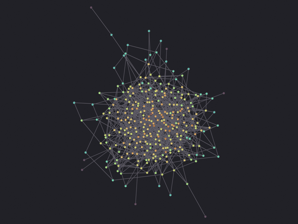
Preferential attachment produces a handful of hubs with a degree many times the median. Mapped linearly they take the top of the scale and everything else is compressed into the bottom stop: a degree of 2 is indistinguishable from a degree of 10. The second render clips the top 2 %.

scale_free = GRAPHS["scale_free"]
sf_csv = write_edge_csv(scale_free, OUT / "scale_free_edges.csv")
sf = import_edge_list(sf_csv, "ScaleFree")
sf_degree = np.array([float(scale_free.degree(int(n))) for n in node_names(sf)])
set_point_attribute(sf, "degree", sf_degree)

cut = np.percentile(sf_degree, 98)
above = int((sf_degree > cut).sum())
print(f"degrees: median {np.median(sf_degree):g}, 98th percentile {cut:.1f}, "
      f"max {sf_degree.max():g}")
print(f"{len(sf_degree) - above} of {len(sf_degree)} nodes sit below the 98th "
      f"percentile, i.e. inside the bottom {cut / sf_degree.max() * 100:.0f} % "
      f"of a linear ramp")
print(f"the remaining {above} nodes have the other "
      f"{100 - cut / sf_degree.max() * 100:.0f} % to themselves")

Info: Loaded 2 columns
Loading graph from notebooks/out/15_abstract/scale_free_edges.csv...
  CSV read in 0.00s
  Edges extracted in 0.00s
  Nodes extracted in 0.00s
Total load time: 0.00s
  Nodes: 300, Edges: 596

Creating graph object with 300 nodes...
  Random positions generated in 0.00s (seed=1426602425)
  Vertices created in 0.00s
  596 edges created in 0.00s
  Mesh conversion in 0.00s
  Object created in 0.00s
DataFrame columns: ['source', 'target']
DataFrame shape: (596, 2)
Source column: source, Target column: target
Number of mesh vertices: 300
Number of mesh edges: 596
Selected attributes for import: ['source', 'target']
Imported 0 attribute columns
  Attributes imported in 0.00s
Total graph creation time: 0.00s

======================================================================
Layout algorithm: SPRING
Graph: 300 nodes, 596 edges
Parameters:
  - algorithm: SPRING
  - iterations: 50
  - scale: 5.0000
  - num_nodes: 300
  - num_edges: 596
Execution time: 0.106s
Status: success
======================================================================

Info: Auto-layout applied: SPRING
Info: Graph created: 300 nodes, 596 edges (SPRING layout applied)
degrees: median 3, 98th percentile 14.0, max 55
294 of 300 nodes sit below the 98th percentile, i.e. inside the bottom 25 % of a linear ramp
the remaining 6 nodes have the other 75 % to themselves

path = nb.render(sf, "renders/01_abstract/5_scale_free_linear",
                 look='ink', color_attribute="degree",
                 node_fraction=0.28, verbose=False)
print("unclipped, the ramp maps", sg.render.color_range(sf))
nb.show(path)
nb.check_render(path)

Info: Geometry Nodes modifier added
Info: Attribute -> degree  ·  degree -> turbo [log]  [2 … 55] on Point
unclipped, the ramp maps (2.0, 55.0)

[PASS] 5_scale_free_linear.png legible — 21.3% ink (healthy range 0.5–60%)

True

path = nb.render(sf, "renders/01_abstract/6_scale_free_clipped",
                 look='ink', color_attribute="degree",
                 clip_high_pct=98, node_fraction=0.28,
                 verbose=False)
print("clipped at 98 %, the ramp maps", sg.render.color_range(sf))
nb.show(path)
nb.check_render(path)

Info: Geometry Nodes modifier added
Info: Attribute -> degree  ·  degree -> turbo [log]  [2 … 14.02] on Point
clipped at 98 %, the ramp maps (2.0, 14.020000457763672)

[PASS] 6_scale_free_clipped.png legible — 21.3% ink (healthy range 0.5–60%)

True

The two frames have the same geometry, the same node size and the same ink to within a tenth of a percent. check_render cannot tell them apart and neither can any other automatic test here. Only one can be read, which is the argument for looking at every figure.

print(f"unclipped ink {nb.ink(nb.out('renders/01_abstract/5_scale_free_linear.png')) * 100:.1f} %")
print(f"clipped   ink {nb.ink(nb.out('renders/01_abstract/6_scale_free_clipped.png')) * 100:.1f} %")
sf.hide_render = True

unclipped ink 21.3 %
clipped   ink 21.3 %

7 · A matrix somebody else made: SuiteSparse

Everything so far was generated on this machine. The SuiteSparse Matrix Collection (https://sparse.tamu.edu) is about 3,000 real sparse matrices from structural engineering, circuit simulation, optimization and web crawls; scigraphs.download_suitesparse turns one into a graph.

RUN_SUITESPARSE is off by default: the only cell that reaches the network. On, it costs

• one GET https://sparse.tamu.edu/MM/<Group>/<Name>.tar.gz (SciGraphs/core/data_io/suitesparse_importer.py:65), 120 s timeout;
• no caching: the importer downloads into memory, extracts the .mtx and drops the archive, so every run pays the transfer again;
• the default Grund/bayer09 is one of the small ones; the collection goes up to hundreds of millions of non-zeros, with no warning before fetching one.

scigraphs.browse_suitesparse is not an API: it is webbrowser.open("https://sparse.tamu.edu") and nothing else (SciGraphs/ui/operators/scigraphs/suitesparse_operators.py:66), so the catalog cannot be searched from the add-on; pick the identifier in a browser and paste it in. Under blender -b it would try to spawn a browser, the second reason for the switch.

RUN_SUITESPARSE = False

SUITESPARSE_ID = "Grund/bayer09"

Two settings decide what graph comes out of a matrix that is not necessarily square or symmetric:

• suitesparse_mode='BIPARTITE' (default) makes a node per row and per column, named R<i> and C<j>, with an edge per non-zero. It preserves the matrix exactly and lays out long and thin.
• suitesparse_mode='SYMMETRIC' reads the matrix as an adjacency matrix, symmetrizing it as A + Aᵀ. Only defensible when rows and columns index the same thing.
• suitesparse_giant_only=True keeps the largest connected component. Real solver matrices are full of tiny detached fragments, and a layout spends most of its frame separating them from the part you wanted.

A few matrices ship a <name>_coord.mtx alongside, and the importer then uses those coordinates as the initial positions (suitesparse_importer.py:246): the one case here where an abstract graph arrives with a geometry of its own.

if RUN_SUITESPARSE:
    props = bpy.context.scene.scigraphs
    props.suitesparse_id = SUITESPARSE_ID
    props.suitesparse_mode = 'BIPARTITE'
    props.suitesparse_giant_only = True
    props.auto_layout_on_import = True
    props.layout_algorithm = 'SPRING'
    props.layout_scale = 5.0
    np.random.seed(LAYOUT_SEED)

    result = bpy.ops.scigraphs.download_suitesparse()
    print("download_suitesparse ->", result)
    print("status:", props.suitesparse_status)

    if 'FINISHED' in result:
        matrix_obj = bpy.context.active_object
        matrix_obj.name = "SuiteSparse"
        set_point_attribute(
            matrix_obj, "degree",
            np.bincount(edge_pairs(matrix_obj).ravel(),
                        minlength=len(matrix_obj.data.vertices)).astype(float))
        nb.figure(matrix_obj, "renders/01_abstract/7_suitesparse",
                  look='ink', color_attribute="degree",
                  clip_high_pct=98, node_fraction=0.28)
else:
    print(f"RUN_SUITESPARSE is off. It would fetch "
          f"https://sparse.tamu.edu/MM/{SUITESPARSE_ID}.tar.gz, "
          f"uncached, on every run.")

RUN_SUITESPARSE is off. It would fetch https://sparse.tamu.edu/MM/Grund/bayer09.tar.gz, uncached, on every run.

8 · Saving

The CSVs are what create_graph reads, so a saved edge list plus the two seeds at the top of this notebook rebuilds every figure above.

print("written to", nb.rel(OUT))
for path in sorted(OUT.iterdir()):
    print(f"   {path.name:<34} {path.stat().st_size / 1e3:6.1f} kB")

check("the graphs can be rebuilt from what was saved",
      (OUT / "karate_edges.csv").is_file()
      and (OUT / "scale_free_edges.csv").is_file())

written to notebooks/out/15_abstract
   comma_labels.csv                      0.0 kB
   innocent_column_names.csv             0.2 kB
   karate_edges.csv                      0.4 kB
   karate_node_attributes.tsv            0.6 kB
   random_edges.csv                      6.5 kB
   scale_free_edges.csv                  3.9 kB
   small_world_edges.csv                 6.6 kB
   small_world_from_matrix.csv           5.1 kB
[PASS] the graphs can be rebuilt from what was saved

True

Rendering

Seven figures, all EEVEE through sg.render; notebook 13 explains the render path. Elsewhere the overhead camera is there so a map can be measured off the page; here nothing can be, and the reason to keep it is that it is the only projection under which the same layout gives the same picture twice, which comparing figures 5 and 6, or 1 and 3, depends on. Notebook 02 examines the trade properly.

The Vulkan warning applies here as everywhere: on Blender’s Vulkan backend, the default on Linux, gpu.state.point_size_set does nothing for the add-on’s shaders, so POINT and DISK nodes in the interactive preview come out 1 pixel wide. Start Blender with --gpu-backend opengl for any render you intend to look at.

Summary

Five defects, all in the add-on, with the workaround used here:

What	Where	Workaround used here
density read as a latitude, so the import silently becomes geospatial	core/geo/geospatial.py:40, via data_operators.py:127	use_geospatial = False after load_columns
The 2D/3D spring layouts take no seed	core/mesh/layouts/networkx_layouts.py:8, :18	seed np.random before the operator
Every layout wipes EDGE attributes via rebuild_edges	core/mesh/geometry.py:1227; called from data_operators.py:41 and five places in layout_operators.py	write edge attributes after the layout
Node identifiers are a comma-joined string	core/mesh/geometry.py:383, :394	no commas in node names
create_graph_object links into bpy.context.collection unchecked	core/mesh/geometry.py:376	go through the operator, which supplies a context

Next: 16 · Layouts, the algorithm that invents the positions.