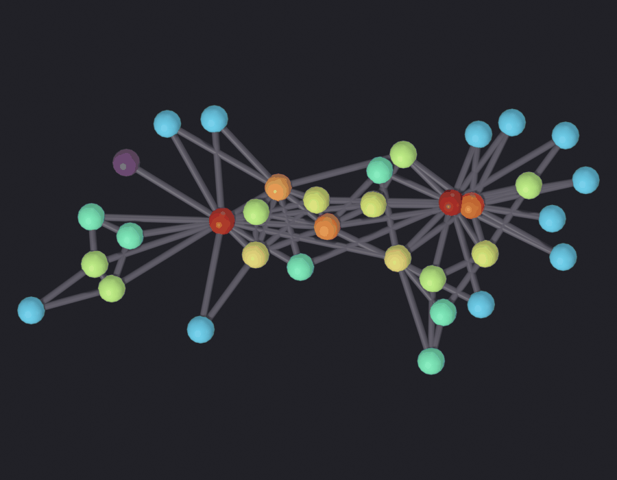
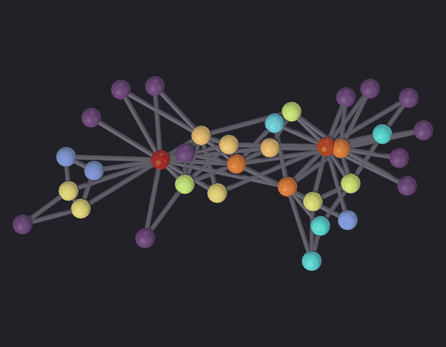
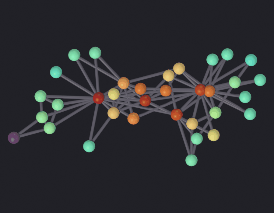
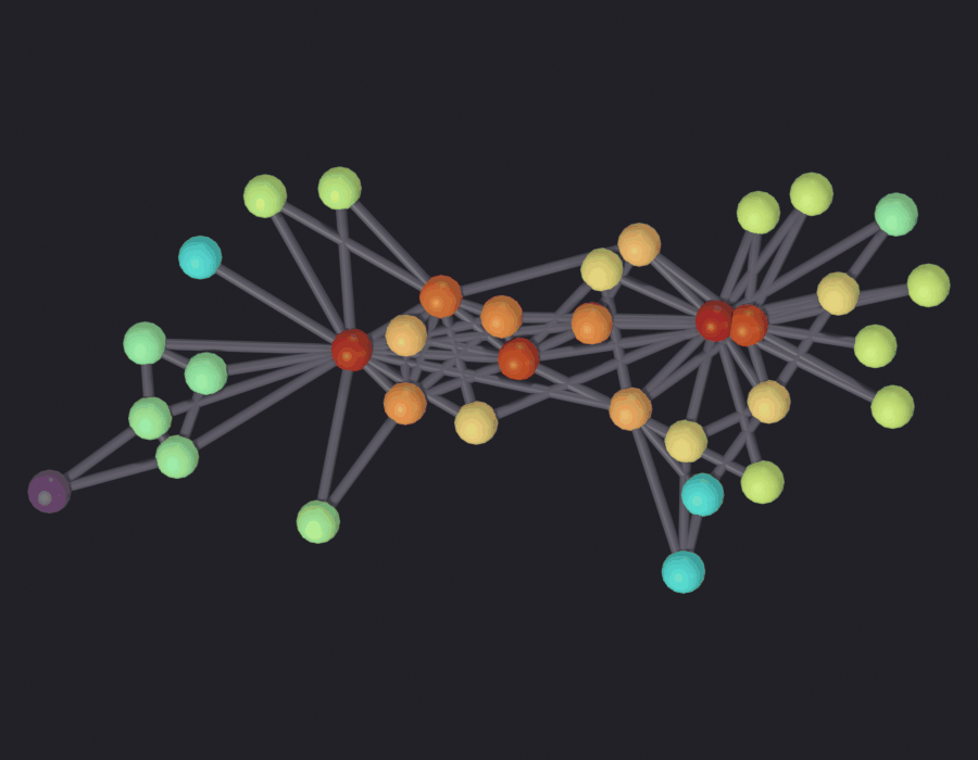
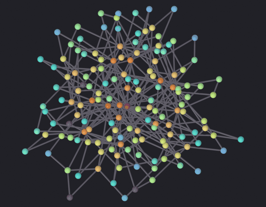
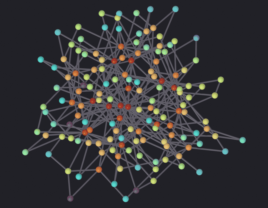
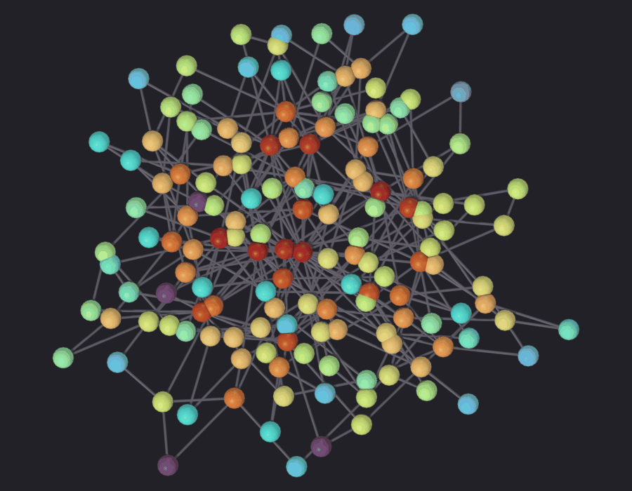
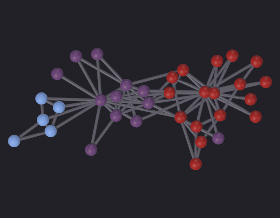
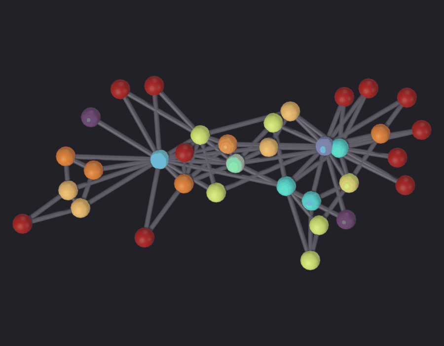
Four centralities on the same graph, and the interesting figure is where they disagree. On Zachary’s karate club, eigenvector and betweenness correlate at 0.694, the weakest pair in the set; closeness spans a factor of two where degree spans seventeen.
The community half is judged, not just displayed. Against the faction split Zachary recorded, only one of the three detected groups is pure and two members land on the wrong side; seven backends give partitions of 3, 5, 7, 12, 17 and 19 groups, ranked differently by modularity and by surprise. Three of the interface controls do not work: the resolution parameter never reaches the detection, the seed is accepted and unused, and the default backend does not return at all on a thirty-four-node graph.
03 · Centrality, clustering and communities
Six SciGraphs operators answer which nodes matter, and which nodes belong together:
Several do something other than what their label says, and one cannot be run at all with its default settings.
The graphs are abstract and seeded, from NetworkX generators: Zachary’s karate club, a Barabási-Albert graph and a directed scale-free graph. No network access, no maps; 18 is the geospatial case study. 15 gets graphs into Blender, 16 lays them out, 18 does paths, trees and flows, 19 does topology.
0 · Setup
import pathlibimport sysdef find_repo():"""Locate the SciGraphs repository, without relying on the cwd. In a normal Jupyter the kernel starts per notebook with the cwd set to its folder. Not here: the kernel lives inside Blender and existed before you opened anything, so the cwd is wherever Blender was launched from. What the extension does know is which folder it is serving to JupyterLab. """ candidates = []try:import bpy prefs = bpy.context.preferences.addons["bl_ext.user_default.jupyter_blender"].preferences candidates.append(pathlib.Path(bpy.path.abspath(prefs.notebook_dir)))exceptException:pass candidates.append(pathlib.Path.cwd())for base in candidates:for directory in (base, *base.parents):if (directory /"SciGraphs"/"api"/"graphs.py").is_file():return directoryraiseRuntimeError("Cannot find the SciGraphs repository. Point at it by hand:\n"" sys.path.insert(0, '/path/to/SciGraphs-1/notebooks/tools')")sys.path.insert(0, str(find_repo() /"notebooks"/"tools"))import itertoolsimport jsonimport bpyimport networkx as nximport numpy as npfrom scipy.stats import spearmanr# `nb` must import first: it puts this repository on sys.path, so the# `SciGraphs` import below reads this tree, not the copy Blender installed.import nbfrom nb import checkfrom SciGraphs import api as sgfrom scigraphs_core import analysisfrom scigraphs_core.mesh.mesh_utils import parse_graph_data_filteredsg.graphs.clear_scene(keep_anchor=False)# Without this wheel `detect_communities` falls back to networkx greedy# modularity and every partition from section 9 on changes.try:import pysurprise # noqa: F401 HAVE_PYSURPRISE =TrueexceptImportError: HAVE_PYSURPRISE =Falsecheck("the pySurprise community backends are installed", HAVE_PYSURPRISE,"without them section 9 measures the networkx fallback instead")
[PASS] the pySurprise community backends are installed — without them section 9 measures the networkx fallback instead
True
1 · Three graphs, built once and never moved
These operators want a graph object: a mesh whose vertices are the nodes and whose mesh.edges are the edges, with num_nodes / num_edges / is_directed as custom properties. That is the mesh-native format scripts/showcase/build_showcase.py writes; the legacy alternative is the nodes_data / edges_data name strings from the GeoDataFrame importers. parse_graph_data_filtered() reads both, and every analysis operator goes through it.
Positions are computed once and reused, so a node lands in the same place on all ten plates. nx.spring_layout is seeded here; the add-on’s default layout is not (SciGraphs/core/mesh/layouts/networkx_layouts.py:8 and :18 call it with no seed=).
Nothing lays the graph out after it is built. The layout operators go through rebuild_edges, which deletes and recreates every mesh edge (SciGraphs/core/mesh/geometry.py:1227 to :1248), taking any EDGE-domain attribute with it. Everything here is node-valued and would survive, but import, lay out, then measure is the safe order in general.
def to_blender(graph, name, seed, spread, directed=False, coll="Abstract"):"""A NetworkX graph as a mesh-native SciGraphs object, laid out once.""" order =list(graph.nodes()) index = {node: i for i, node inenumerate(order)} positions = nx.spring_layout(graph.to_undirected(), seed=seed) coords = np.array([[positions[n][0] * spread, positions[n][1] * spread, 0.0]for n in order], dtype=np.float32) edges = np.array([[index[u], index[v]] for u, v in graph.edges()], dtype=np.int32) mesh = bpy.data.meshes.new(name) mesh.vertices.add(len(order)) mesh.vertices.foreach_set("co", coords.ravel()) mesh.edges.add(len(edges)) mesh.edges.foreach_set("vertices", edges.ravel()) mesh.update() obj = bpy.data.objects.new(name, mesh) obj["num_nodes"] =len(order) obj["num_edges"] =len(edges) obj["is_directed"] =bool(directed) obj["node_names"] = json.dumps([str(n) for n in order]) sg.graphs.collection(coll).objects.link(obj)return obj, orderKARATE = nx.karate_club_graph()karate, karate_order = to_blender(KARATE, "Karate", seed=7, spread=10.0)SCALEFREE = nx.barabasi_albert_graph(150, 2, seed=17)scalefree, scalefree_order = to_blender(SCALEFREE, "BarabasiAlbert", seed=11, spread=13.0)DIRECTED = nx.DiGraph(nx.scale_free_graph(120, seed=4))DIRECTED.remove_edges_from(nx.selfloop_edges(DIRECTED))directed, directed_order = to_blender(DIRECTED, "DirectedScaleFree", seed=5, spread=12.0, directed=True)for obj in (karate, scalefree, directed):print(f"{obj.name:20}{obj['num_nodes']:>4} nodes {obj['num_edges']:>4} edges "f"directed={bool(obj['is_directed'])}")
The operators see only what parse_graph_data_filtered() reconstructs from the mesh. Edge order survives: Blender stores a mesh edge as the ordered pair it was given.
parsed = {obj.name: parse_graph_data_filtered(obj)for obj in (karate, scalefree, directed)}check("the mesh round-trips every node and edge",all(len(parsed[o.name].nodes) == o["num_nodes"]andlen(parsed[o.name].edges) == o["num_edges"]for o in (karate, scalefree, directed)))oriented =sum(1for (a, b), (u, v)inzip(parsed["DirectedScaleFree"].edges, DIRECTED.edges())if (a, b) == (str(u), str(v)))check("edge direction survives the mesh", oriented == DIRECTED.number_of_edges(),f"{oriented}/{DIRECTED.number_of_edges()} pairs in the original order")
[PASS] the mesh round-trips every node and edge
[PASS] edge direction survives the mesh — 197/197 pairs in the original order
True
2 · What calculate_centrality actually computes
Four methods (analysis_operators.py:26 to :35, scene property at splitter_properties.py:229), each a one-line call into NetworkX. The interesting part is the two lines above them:
G = nx.Graph() # analysis.py:16G.add_nodes_from(range(len(graph_data.nodes)))
nx.Graph, unconditionally, whatever is_directed says, so a directed graph is silently symmetrized; section 6 measures the cost. And no weights: edges go in as bare index pairs, because GraphData carries only nodes, edges and an optional dataframe (SciGraphs/core/algorithms/graph.py:3). So betweenness counts shortest paths in hops and closeness is a hop distance, on every graph, always. On a street network, where edge lengths are the entire point, that is not the quantity the label implies.
degree: neighbors over n - 1, and free to compute.
betweenness: the share of all shortest paths passing through the node. A bridge scores high on two neighbors.
closeness: reciprocal of the mean hop distance to everyone else.
eigenvector: degree, weighted recursively by the neighbors’ scores.
sg.graphs.activate(karate)METHODS = ("degree", "betweenness", "closeness", "eigenvector")for method in METHODS: result = bpy.ops.scigraphs.calculate_centrality(method=method)print(f"{method:14}{'/'.join(result):10} -> centrality_{method}")print("\nattributes on", karate.name)for name, domain, dtype in sg.graphs.attributes(karate):ifnot name.startswith("."):print(f" {name:<26}{domain:<7}{dtype}")
Info: Centrality 'degree' calculated
degree         FINISHED   ->  centrality_degree
Info: Centrality 'betweenness' calculated
betweenness    FINISHED   ->  centrality_betweenness
Info: Centrality 'closeness' calculated
closeness      FINISHED   ->  centrality_closeness
Info: Centrality 'eigenvector' calculated
eigenvector    FINISHED   ->  centrality_eigenvector

attributes on Karate
  position                   POINT   FLOAT_VECTOR
  centrality_degree          POINT   FLOAT
  centrality_betweenness     POINT   FLOAT
  centrality_closeness       POINT   FLOAT
  centrality_eigenvector     POINT   FLOAT
The values come from the core function, so the notebook can do arithmetic with them. They match NetworkX exactly: the operator adds a Blender attribute and changes nothing.
karate_gd = parsed["Karate"]centrality = {m: np.array(analysis.calculate_centrality(karate_gd, method=m))for m in METHODS}reference = np.array([nx.betweenness_centrality(KARATE)[n] for n in karate_order])check("betweenness matches networkx on the original graph",float(np.abs(centrality["betweenness"] - reference).max()) <1e-12,f"largest disagreement {np.abs(centrality['betweenness'] - reference).max():.2e}")check("the operator wrote one value per vertex",len(karate.data.attributes["centrality_betweenness"].data)==len(karate.data.vertices))print(f"\n{'measure':<14}{'min':>9}{'median':>9}{'mean':>9}{'max':>9}{'max/med':>9}")for method in METHODS: v = centrality[method]print(f"{method:<14}{v.min():9.4f}{np.median(v):9.4f}{v.mean():9.4f} "f"{v.max():9.4f}{v.max() /max(np.median(v), 1e-12):9.1f}")
[PASS] betweenness matches networkx on the original graph — largest disagreement 0.00e+00
[PASS] the operator wrote one value per vertex

measure              min    median      mean       max   max/med
degree            0.0303    0.0909    0.1390    0.5152       5.7
betweenness       0.0000    0.0026    0.0440    0.4376     170.6
closeness         0.2845    0.3837    0.4265    0.5690       1.5
eigenvector       0.0236    0.1020    0.1464    0.3734       3.7
3 · The four measures, one figure each
Every figure here is an EEVEE render straight down through an orthographic camera, look='ink', colormap turbo: the style notebooks 00 to 09 share, so plates can be laid side by side. Color always carries a quantity this notebook computed, named in color_attribute=, and the node radius is derived from the graph rather than left at the default.
The orthographic frame is solved iteratively, not in one
call
The first EEVEE render of a session comes out cropped, the outermost nodes cut in half by the frame edge. sg.render.frame_camera solves the orthographic scale with Object.camera_fit_coords, which does not reach the answer in one pass from Blender’s default ortho_scale of 6. Repeated calls on the karate graph give an increasing sequence, within a percent of its limit by the third. It bites once per camera; settling the frame first costs nothing.
def settle_camera(obj, resolution, node_fraction=None, edge_ratio=None, rounds=4, report=False):"""Call the framing until the orthographic scale stops moving.""" scene = bpy.context.scene scene.render.resolution_x, scene.render.resolution_y = resolution sg.render.autoscale_geometry( obj, node_fraction=(sg.render.NODE_FRACTION if node_fraction isNoneelse node_fraction), edge_ratio=edge_ratio, verbose=False) scales = []for _ inrange(rounds): cam = sg.render.frame_camera(obj, view='TOP') scales.append(round(float(cam.data.ortho_scale), 3))if report:print(" ortho_scale over four calls:", scales)print(f" the first is {(1- scales[0] / scales[-1]) *100:.0f}% short "f"of the settled value")return scalesPLATE = (900, 700)settle_camera(karate, PLATE, report=True)
  ortho_scale over four calls: [19.792, 19.792, 19.792, 19.792]
  the first is 0% short of the settled value
[19.792, 19.792, 19.792, 19.792]
How much of the ink carries the measurement
nb.check_render measures the fraction of the frame with anything in it at all, which on these figures is dominated by the edge tubes. A node-valued colormap reaching a sixth of the drawn pixels is a figure about wiring. So a second number goes under every plate: the share of drawn pixels that is saturated, i.e. came out of turbo rather than the neutral tube color. It decides node_fraction on the dense figures in sections 5 and 6.
def color_share(path):"""(ink fraction, share of the ink that carries a colormap value)."""from PIL import Image rgb = np.asarray(Image.open(str(path)).convert("RGB"), dtype=np.float32) drawn = np.abs(rgb - rgb.reshape(-1, 3)[0]).sum(axis=2) >24 saturation = np.asarray(Image.open(str(path)).convert("HSV"), dtype=np.float32)[..., 1] /255.0returnfloat(drawn.mean()), float((drawn & (saturation >0.35)).sum()/max(drawn.sum(), 1))def figure(obj, path, resolution=PLATE, node_fraction=None, edge_ratio=None,**kwargs):"""Settle the frame, render, show, check, and report the color share. Returns nothing, for the reason `nb.figure` does not: a cell whose last statement is a call echoes that value into the stored output, and a `PosixPath` would put an absolute home directory into every published copy. """ settle_camera(obj, resolution, node_fraction=node_fraction, edge_ratio=edge_ratio) written = nb.render( obj, path, resolution=resolution, look='ink', verbose=False, node_fraction=(sg.render.NODE_FRACTION if node_fraction isNoneelse node_fraction), edge_ratio=edge_ratio, **kwargs) nb.show(written) nb.check_render(written) ink, colored = color_share(written)print(f" {ink *100:.1f}% ink, of which {colored *100:.0f}% carries the colormap")returnNone
Four plates of the same 34 nodes in the same positions. Read each against the distribution printed above it: the color is a linear ramp between the ends of the mapped range, and without the spread the ramp is decoration.
for method in METHODS: v = centrality[method]print(f"\n{method} "+" ".join(f"p{p}={q:.4f}"for p, q inzip((0, 25, 50, 75, 90, 100), np.percentile(v, [0, 25, 50, 75, 90, 100])))) figure(karate, f"renders/03_centrality/1_karate_{method}", color_attribute=f"centrality_{method}")
[PASS] 1_karate_degree.png legible — 15.4% ink (healthy range 0.5–60%)
  15.4% ink, of which 41% carries the colormap

betweenness   p0=0.0000  p25=0.0000  p50=0.0026  p75=0.0319  p90=0.1420  p100=0.4376
Info: Geometry Nodes modifier added
Info: Attribute -> centrality_betweenness  ·  centrality_betweenness -> turbo [log]  [0 … 0.4376] on Point
[PASS] 1_karate_betweenness.png legible — 15.3% ink (healthy range 0.5–60%)
  15.3% ink, of which 40% carries the colormap

closeness   p0=0.2845  p25=0.3718  p50=0.3837  p75=0.4802  p90=0.5334  p100=0.5690
Info: Geometry Nodes modifier added
Info: Attribute -> centrality_closeness  ·  centrality_closeness -> turbo [log]  [0.2845 … 0.569] on Point
[PASS] 1_karate_closeness.png legible — 15.4% ink (healthy range 0.5–60%)
  15.4% ink, of which 37% carries the colormap

eigenvector   p0=0.0236  p25=0.0807  p50=0.1020  p75=0.1870  p90=0.2958  p100=0.3734
Info: Geometry Nodes modifier added
Info: Attribute -> centrality_eigenvector  ·  centrality_eigenvector -> turbo [log]  [0.02363 … 0.3734] on Point
[PASS] 1_karate_eigenvector.png legible — 15.4% ink (healthy range 0.5–60%)
  15.4% ink, of which 36% carries the colormap
Every measure finds the two factions the club actually split into: the instructor’s node and the president’s node are the extremes of all four plates. What separates the measures is everything in between.
Betweenness is also the only one whose low end is a hard zero for a large part of the graph. Those nodes lie on no shortest path between any other pair, so they share the bottom stop of the ramp and cannot be told apart.
for method in METHODS:print(f"nodes at exactly zero {method:<12}: "f"{int((centrality[method] ==0).sum()):>3} of {len(karate_order)}")
nodes at exactly zero degree      :   0 of 34
nodes at exactly zero betweenness :  12 of 34
nodes at exactly zero closeness   :   0 of 34
nodes at exactly zero eigenvector :   0 of 34
4 · Where the measures disagree
Where the four plates differ, as a rank correlation table. Spearman’s ρ, because none of these measures is on a comparable scale and only the ordering matters.
def rank_table(values, label, width=11):"""Print the Spearman matrix and return it as {(a, b): rho}.""" keys =list(values) pad =max(len(k) for k in keys) +2print(f"Spearman rank correlation: {label}")print(" "* pad +"".join(f"{k[:width -1]:>{width}}"for k in keys)) matrix = {}for a in keys: row = []for b in keys: rho =float(spearmanr(values[a], values[b]).statistic) matrix[(a, b)] = rho row.append(f"{rho:{width}.3f}")print(f"{a:<{pad}}"+"".join(row))return matrixkarate_rho = rank_table(centrality, "Zachary's karate club (34 nodes)")
Degree and betweenness agree at ρ ≈ 0.90 and still disagree about individual nodes, which is why both exist.
Eigenvector is the odd one out: ρ ≈ 0.69 against betweenness, its lowest pairing, ≈ 0.86 against closeness, its highest. It rewards being near the dense core; betweenness rewards being between things.
Closeness correlates with everything (≈ 0.86 to 0.90) and is the least informative column for that reason. On a graph of diameter 5 a mean hop distance has little room to vary: it spans a factor of two, against a factor of infinity for betweenness.
off_diagonal = {k: v for k, v in karate_rho.items() if k[0] != k[1]}lowest =min(off_diagonal, key=off_diagonal.get)check("eigenvector and betweenness are the least similar pair",set(lowest) == {"eigenvector", "betweenness"},f"{lowest[0]} vs {lowest[1]}, rho = {off_diagonal[lowest]:.3f}")closeness_span = centrality["closeness"].max() / centrality["closeness"].min()degree_span = centrality["degree"].max() / centrality["degree"].min()check("closeness has the narrowest range of the four", closeness_span < degree_span,f"closeness spans x{closeness_span:.1f}, degree x{degree_span:.1f}")
[PASS] eigenvector and betweenness are the least similar pair — betweenness vs eigenvector, rho = 0.694
[PASS] closeness has the narrowest range of the four — closeness spans x2.0, degree x17.0
True
The nodes betweenness ranks highly that degree does not
A node with two or three neighbors and a high betweenness is a bridge: cut it and the graph falls in two. Degree cannot see that.
def rank_of(values):"""1-based rank, highest value first."""return (-np.asarray(values)).argsort().argsort() +1rank_degree = rank_of(centrality["degree"])rank_between = rank_of(centrality["betweenness"])climb = rank_degree - rank_betweenprint(f"{'node':>5}{'degree':>8}{'rank':>5}{'betweenness':>12}{'rank':>5} "f"{'climb':>6}{'neighbors':>11}")for i in np.argsort(-climb)[:6]: node = karate_order[i]print(f"{node:>5}{centrality['degree'][i]:8.4f}{rank_degree[i]:5d} "f"{centrality['betweenness'][i]:12.4f}{rank_between[i]:5d} "f"{climb[i]:+6d}{KARATE.degree(node):11d}")bridge =int(np.argmax(climb))print(f"\nnode {karate_order[bridge]} has {KARATE.degree(karate_order[bridge])} "f"neighbors and is ranked {rank_between[bridge]} of {len(karate_order)} "f"by betweenness, against {rank_degree[bridge]} by degree")check("betweenness promotes a low-degree bridge over higher-degree nodes", climb.max() >=5, f"largest climb {climb.max():+d} places")
 node   degree  rank  betweenness  rank  climb   neighbors
   19   0.0909    18       0.0325     9     +9           3
   14   0.0606    32       0.0000    24     +8           2
    5   0.1212    15       0.0300    10     +5           4
    8   0.1515    10       0.0559     6     +4           5
    9   0.0606    23       0.0008    20     +3           2
    6   0.1212    14       0.0300    11     +3           4

node 19 has 3 neighbors and is ranked 9 of 34 by betweenness, against 18 by degree
[PASS] betweenness promotes a low-degree bridge over higher-degree nodes — largest climb +9 places
True
5 · Distributions, and why clip_high_pct exists
The karate club is small enough for a linear ramp. barabasi_albert_graph(150, 2) grows by preferential attachment, so its degree distribution has a heavy tail by construction, and its betweenness distribution is heavier still: a hub is the only route between the branches hanging off it.
sg.graphs.activate(scalefree)for method in ("degree", "betweenness"): bpy.ops.scigraphs.calculate_centrality(method=method)sf_gd = parsed["BarabasiAlbert"]sf = {m: np.array(analysis.calculate_centrality(sf_gd, method=m))for m in ("degree", "betweenness")}for method, values in sf.items(): order = np.sort(values)[::-1]print(f"\n{method}")print(" "+" ".join(f"p{p}={np.percentile(values, p):.5f}"for p in (50, 75, 90, 95, 98, 99, 100)))print(f" top 3 nodes hold {order[:3].sum() / values.sum() *100:5.1f}% of the total")print(f" max / median x{values.max() / np.median(values):.0f}")skew = {m: v.max() / np.median(v) for m, v in sf.items()}check("betweenness is far more skewed than degree", skew["betweenness"] >3* skew["degree"],f"x{skew['betweenness']:.0f} against x{skew['degree']:.0f}")
Info: Centrality 'degree' calculated
Info: Centrality 'betweenness' calculated

degree
  p50=0.02013  p75=0.03188  p90=0.04698  p95=0.07081  p98=0.08738  p99=0.10423  p100=0.18792
  top 3 nodes hold  10.0% of the total
  max / median      x9

betweenness
  p50=0.00443  p75=0.01492  p90=0.03855  p95=0.06890  p98=0.09626  p99=0.11633  p100=0.36246
  top 3 nodes hold  24.6% of the total
  max / median      x82
[PASS] betweenness is far more skewed than degree — x82 against x9
True
Mapped linearly, that puts one node at the top of turbo and compresses the other 149 into the bottom. The percentile clip is the only fix that works here.
vmin= and vmax= are silently ineffective.scigraphs.color_set_attribute calls fn.update_property_range(props, obj, target) immediately before apply_coloring (SciGraphs/ui/coloring/operators.py:374), overwriting both with the attribute’s own extremes. Nothing is reported. Two centralities cannot be put on one shared absolute scale through this path.
The graph needs its visualization built before the coloring operator has anything to wire into, which render_eevee normally does on the way past.
sg.render.autoscale_geometry(scalefree, node_fraction=0.35, verbose=False)sg.render.material(scalefree)sg.render.geometry_nodes(scalefree)sg.render.color_graph(scalefree, "centrality_betweenness", colormap="turbo", vmin=0.0, vmax=1.0, verbose=False)applied = sg.render.color_range(scalefree)print("asked for vmin/vmax (0.0, 1.0)")print(f"actually mapped ({applied[0]:.6f}, {applied[1]:.6f})")print(f"attribute extremes ({sf['betweenness'].min():.6f}, "f"{sf['betweenness'].max():.6f})")check("vmin/vmax were overwritten by the attribute's own range",abs(applied[1] - sf["betweenness"].max()) <1e-4,"clip_low_pct / clip_high_pct are the controls that work")
Info: Geometry Nodes modifier added
Info: Attribute -> centrality_betweenness  ·  centrality_betweenness -> turbo [log]  [0 … 0.3625] on Point
asked for vmin/vmax  (0.0, 1.0)
actually mapped      (0.000000, 0.362459)
attribute extremes   (0.000000, 0.362459)
[PASS] vmin/vmax were overwritten by the attribute's own range — clip_low_pct / clip_high_pct are the controls that work
True
Three plates, one variable at a time. First the defaults: a linear ramp over the raw range and the house node_fraction of 0.35.
Info: Geometry Nodes modifier added
Info: Attribute -> centrality_betweenness  ·  centrality_betweenness -> turbo [log]  [0 … 0.3625] on Point
[PASS] 2_ba_default.png legible — 26.5% ink (healthy range 0.5–60%)
  26.5% ink, of which 26% carries the colormap
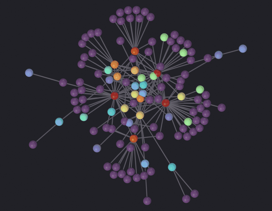
One warm node and a field of purple. Correct, and it says only “there is a hub”. Now the clip alone, at the 98th percentile, sizing unchanged.
print(f"clipping at p98 = {np.percentile(sf['betweenness'], 98):.5f}, "f"against a maximum of {sf['betweenness'].max():.5f}")figure(scalefree, "renders/03_centrality/3_ba_clip98", color_attribute="centrality_betweenness", clip_high_pct=98)
clipping at p98 = 0.09626, against a maximum of 0.36246
Info: Geometry Nodes modifier added
Info: Attribute -> centrality_betweenness  ·  centrality_betweenness -> turbo [log]  [0 … 0.09626] on Point
[PASS] 3_ba_clip98.png legible — 26.5% ink (healthy range 0.5–60%)
  26.5% ink, of which 27% carries the colormap
The ramp is now spent on the 98 % of the graph the first plate threw away, and the tree-like periphery becomes readable: chains of blue out to the leaves are nodes with real betweenness that the linear scale flattened onto the floor. The cost is the top, where every node above the 98th percentile is the same red, so the plate can no longer say which hub is biggest. Hence the percentiles printed above the figure.
nb.check_render cannot adjudicate this. Clipping moves colors around without changing how many pixels carry them, so both plates come back at essentially the same ink.
Then the sizing. At node_fraction=0.35, 150 nodes of mean degree 4 put four tubes in the frame for every sphere. At 0.5, with the tube ratio pinned to 0.12 instead of the derived 0.25, the figure is about the nodes again; the ink fraction barely moves, so the legibility check cannot see it either.
Info: Geometry Nodes modifier added
Info: Attribute -> centrality_betweenness  ·  centrality_betweenness -> turbo [log]  [0 … 0.09626] on Point
[PASS] 4_ba_clip98_sized.png legible — 27.0% ink (healthy range 0.5–60%)
  27.0% ink, of which 52% carries the colormap
6 · Directed against undirected
calculate_directed_centrality refuses to run unless obj["is_directed"] is set (analysis_operators.py:205). Its six methods (splitter_properties.py:242) are PageRank, HITS hub, HITS authority, in-degree, out-degree and Katz. The method comes from scene.scigraphs.directed_centrality_method rather than an operator property, so from a script that scene property is the only way to choose one.
DIRECTED_METHODS = ('pagerank', 'hub_score', 'authority_score','in_degree', 'out_degree', 'katz')sg.graphs.activate(directed)directed_gd = parsed["DirectedScaleFree"]directed_values = {}# Two of the six need this: `nx.hits` starts ARPACK from an unseeded random# vector and nothing in SciGraphs seeds it. Measured after the table.np.random.seed(17)for method in DIRECTED_METHODS: bpy.context.scene.scigraphs.directed_centrality_method = method result = bpy.ops.scigraphs.calculate_directed_centrality() directed_values[method] = np.array( analysis.calculate_directed_centrality(directed_gd, method=method))print(f"{method:16}{'/'.join(result):10} -> directed_{method}")reciprocal =sum(1for u, v in DIRECTED.edges() if DIRECTED.has_edge(v, u))print(f"\nreciprocal edges: {reciprocal} of {DIRECTED.number_of_edges()}; "f"{100* (1- reciprocal / DIRECTED.number_of_edges()):.0f}% of this "f"graph is one-way")
calculate_centrality on the same directed object returns exactly nx.degree_centrality of the underlying undirected graph: direction discarded, reciprocal pairs collapsed onto one edge. No warning, and is_directed is never consulted on that path.
undirected_degree = np.array( analysis.calculate_centrality(directed_gd, method='degree'))symmetrized = np.array([nx.degree_centrality(DIRECTED.to_undirected())[n]for n in directed_order])check("calculate_centrality on a directed graph == the symmetrized graph",float(np.abs(undirected_degree - symmetrized).max()) <1e-12,"`nx.Graph()` at analysis.py:16, whatever is_directed says")rho =float(spearmanr(undirected_degree, directed_values['pagerank']).statistic)print(f"\nSpearman(undirected degree, PageRank) = {rho:.3f}")print("The two orderings share about half their information. On a directed ""graph they answer different questions, and only one of the two ""operators knows the graph is directed.")
[PASS] calculate_centrality on a directed graph == the symmetrized graph — `nx.Graph()` at analysis.py:16, whatever is_directed says

Spearman(undirected degree, PageRank) = 0.565
The two orderings share about half their information. On a directed graph they answer different questions, and only one of the two operators knows the graph is directed.
The rank correlations among the directed measures, with the symmetrized degree as a control column.
SHORT = {'pagerank': 'pagerank', 'hub_score': 'hub', 'authority_score': 'authority','in_degree': 'in_deg', 'out_degree': 'out_deg', 'katz': 'katz'}directed_table = {SHORT[k]: v for k, v in directed_values.items()}directed_table['undirected'] = undirected_degreedirected_rho = rank_table(directed_table,"directed scale-free (120 nodes)", width=10)
PageRank tracks in-degree, not out-degree: a random surfer follows links forward, so it accumulates where links point.
Authority tracks in-degree and hub tracks out-degree, as HITS is defined to do. Each is computed from its own nx.hits(G, max_iter=1000) call (analysis.py:347 and :355), so asking for both runs the same iteration twice and throws half of each result away.
The symmetrized degree correlates decently with everything and matches nothing, which is the argument for a directed operator at all.
One more, undocumented: Katz and PageRank agree to three decimal places here (ρ = 0.999), and both agree with plain in-degree at 0.993. On a graph this sparse (197 edges over 120 nodes, 92 % one-way) the recursive measures have almost nothing to recurse through and all three collapse onto “how many arrows point at me”. They separate on a denser graph; here, running all six costs six iterations and yields three answers.
check("Katz and PageRank agree almost exactly on this sparse graph", directed_rho[('katz', 'pagerank')] >0.99,f"rho = {directed_rho[('katz', 'pagerank')]:.4f}")check("PageRank sits closer to in-degree than to out-degree", directed_rho[('pagerank', 'in_deg')] > directed_rho[('pagerank', 'out_deg')],f"{directed_rho[('pagerank', 'in_deg')]:.3f} against "f"{directed_rho[('pagerank', 'out_deg')]:.3f}")check("hub tracks out-degree and authority tracks in-degree", directed_rho[('hub', 'out_deg')] > directed_rho[('hub', 'in_deg')]and directed_rho[('authority', 'in_deg')] > directed_rho[('authority', 'out_deg')])
[PASS] Katz and PageRank agree almost exactly on this sparse graph — rho = 0.9992
[PASS] PageRank sits closer to in-degree than to out-degree — 0.993 against -0.077
[PASS] hub tracks out-degree and authority tracks in-degree
True
Two of those columns are not reproducible
The hub and authority rows move between runs on the same graph with nothing changed: two consecutive runs rank the nodes at a Spearman ρ well under 1 against each other, a wider gap than the one separating two of the six measures.
NetworkX 3.6 computes HITS as a one-singular-value decomposition, scipy.sparse.linalg.svds(A, k=1, maxiter=..., tol=...), and passes a starting vector only when the caller supplies nstart. SciGraphs calls nx.hits(G, max_iter=1000) with no nstart (analysis.py:347 for hub, :355 for authority), so ARPACK starts from an unseeded random vector.
The values are reproducible to about 1e-16; the ranking is not. Most of this graph has an authority score that is numerically zero, and sorting 88 zeros by their 1e-17 of floating-point noise gives a different order every time. Seeding NumPy’s global RNG immediately before the call pins it.
def hits_authority(): scores = nx.hits(DIRECTED, max_iter=1000)[1]return np.array([scores[n] for n in directed_order])unseeded = [hits_authority() for _ inrange(3)]np.random.seed(17)seeded_a = hits_authority()np.random.seed(17)seeded_b = hits_authority()print(f"authority scores below 1e-12: {int((np.abs(unseeded[0]) <1e-12).sum())} "f"of {len(unseeded[0])} nodes")print(f"largest value difference between two unseeded runs: "f"{np.abs(unseeded[0] - unseeded[1]).max():.1e}")for i in (1, 2):print(f"Spearman(run 0, run {i}) unseeded : "f"{spearmanr(unseeded[0], unseeded[i]).statistic:.3f}")print(f"Spearman(run 0, run 1) seeded : "f"{spearmanr(seeded_a, seeded_b).statistic:.3f}")drift =min(float(spearmanr(unseeded[0], unseeded[i]).statistic) for i in (1, 2))check("unseeded HITS gives the same values in a different order", drift <0.999and np.abs(unseeded[0] - unseeded[1]).max() <1e-12,f"worst rank agreement between two runs: {drift:.3f}")check("seeding numpy before the call makes it reproducible", spearmanr(seeded_a, seeded_b).statistic ==1.0)
authority scores below 1e-12: 88 of 120 nodes
largest value difference between two unseeded runs: 1.4e-16
Spearman(run 0, run 1) unseeded : 0.960
Spearman(run 0, run 2) unseeded : 0.920
Spearman(run 0, run 1) seeded   : 1.000
[PASS] unseeded HITS gives the same values in a different order — worst rank agreement between two runs: 0.920
[PASS] seeding numpy before the call makes it reproducible
True
The in- and out-degree normalization is not the standard
one
nx.in_degree_centrality divides by n - 1, so the value is the fraction of the graph pointing at this node and two graphs can be compared. The operator divides by the largest in-degree in this graph (analysis.py:362 to :363, and :367 to :368 for out-degree), so the busiest node is always exactly 1.0 and the scale is graph-relative. The enum description says only “Number of incoming connections (popularity)”.
It is a rescaling, so the rank table above still holds; an absolute reading of the number does not.
print(f"operator in_degree max = {directed_values['in_degree'].max():.4f}")print(f"networkx in_degree max = {max(nx.in_degree_centrality(DIRECTED).values()):.4f}")check("the operator's in-degree is normalized to its own maximum",abs(directed_values['in_degree'].max() -1.0) <1e-9)
operator in_degree  max = 1.0000
networkx in_degree  max = 0.2773
[PASS] the operator's in-degree is normalized to its own maximum
True
And it divides by zero on an edgeless directed graph.max_in is 0 when nothing has an incoming edge, and the guard above (if in_deg.values() else 1) only catches an empty dict, not a dict of zeros (analysis.py:362 and :367). A directed graph with no edges (a failed import, a filter that matched nothing) raises ZeroDivisionError instead of returning zeros.
class _Edgeless: nodes = [str(i) for i inrange(5)] edges = []try: analysis.calculate_directed_centrality(_Edgeless(), method='in_degree') raised =NoneexceptExceptionas exc: # noqa: BLE001 - the point is which exception raised =type(exc).__name__check("an edgeless directed graph raises rather than returning zeros", raised =="ZeroDivisionError", f"raised {raised}")
[PASS] an edgeless directed graph raises rather than returning zeros — raised ZeroDivisionError
True
PageRank on the directed graph, clipped at the 98th percentile for the same reason the Barabási-Albert plate was: a scale-free in-degree gives a scale-free PageRank.
pagerank = directed_values['pagerank']print("PageRank "+" ".join(f"p{p}={np.percentile(pagerank, p):.4f}"for p in (50, 90, 98, 100)))figure(directed, "renders/03_centrality/5_directed_pagerank", color_attribute="directed_pagerank", clip_high_pct=98, node_fraction=0.5, edge_ratio=0.12)
[PASS] 5_directed_pagerank.png legible — 17.7% ink (healthy range 0.5–60%)
  17.7% ink, of which 47% carries the colormap
There are no arrows in that figure and there cannot be: the tube between two nodes is one piece of swept geometry with no head, so a directed graph and its symmetrization draw identically. Only the color carries the direction.
7 · Strong components, and a cycle count that is not one
find_sccs writes an scc_id per node and the totals onto the object. On a scale-free directed graph almost every component is a single node: the graph grows outward, so there is nothing to come back on.
result = bpy.ops.scigraphs.find_sccs()print("find_sccs", "/".join(result))print(f" components {directed['num_sccs']}")print(f" largest {directed['largest_scc']} nodes")print(f" singletons {sum(1for c in nx.strongly_connected_components(DIRECTED) iflen(c) ==1)}")check("scc_id agrees with networkx", directed["num_sccs"] == nx.number_strongly_connected_components(DIRECTED))
  Rebuilt simple GN tree (attribute stripping updated)
Info: Found 106 strongly connected components, largest: 15 nodes
find_sccs FINISHED
  components   106
  largest      15 nodes
  singletons   105
[PASS] scc_id agrees with networkx
True
detect_patterns writes eight booleans and counts onto the object. Seven are one NetworkX predicate each and are exactly right. The eighth is not.
pattern_num_cycles is capped at 1000, but the cap is applied after enumerating every cycle.analysis.py:411 is cycles = list(nx.simple_cycles(G)), and only the next line slices it to [:1000]. The comment says “Limit to 1000 to avoid performance issues”; the limit avoids nothing. Cycle counts grow super-exponentially with density, so on this 120-node graph the operator materializes a list and then discards part of it, and on a moderately denser one it does not return at all. nx.simple_cycles is a generator and itertools.islice would have made the comment true.
true_cycles =sum(1for _ in itertools.islice(nx.simple_cycles(DIRECTED), 200_000))result = bpy.ops.scigraphs.detect_patterns()print("detect_patterns", "/".join(result))for key insorted(k for k in directed.keys() if k.startswith("pattern_")):print(f" {key[8:]:<36}{directed[key]}")print(f"\nsimple cycles actually enumerated: {true_cycles}")print(f"reported as pattern_num_cycles : {directed['pattern_num_cycles']}")check("the reported cycle count is the cap, not the count", directed["pattern_num_cycles"] ==min(true_cycles, 1000)and true_cycles >1000,f"{true_cycles} enumerated, {directed['pattern_num_cycles']} reported")
Info: 1000 cycles
detect_patterns FINISHED
  has_cycles                           True
  is_dag                               False
  is_forest                            False
  is_strongly_connected                False
  is_tree                              False
  is_weakly_connected                  True
  num_cycles                           1000
  num_strongly_connected_components    106
  num_weakly_connected_components      1

simple cycles actually enumerated: 1210
reported as pattern_num_cycles   : 1000
[PASS] the reported cycle count is the cap, not the count — 1210 enumerated, 1000 reported
True
8 · Two operators called “clustering”, measuring different
things
The naming trap in the panel:
Operator
Question
Answer
calculate_clustering
how cliquey is the neighborhood of this node?
one float per node, in [0, 1]
apply_clustering
which group does this node belong to?
one integer label per node
The first is the local clustering coefficient: of all the pairs of my neighbors, what fraction are joined to each other. The second is community detection. They sit one word apart in the panel, and apply_clustering also writes the coefficient under a third name, node_clustering (analysis_operators.py:170), so the same quantity ends up on the mesh twice.
sg.graphs.activate(karate)print(bpy.ops.scigraphs.calculate_clustering(), "-> 'clustering'")coefficient = np.array(analysis.calculate_clustering(karate_gd))print(f"\nlocal clustering coefficient: min {coefficient.min():.3f} "f"median {np.median(coefficient):.3f} max {coefficient.max():.3f}")print(f"nodes with a fully connected neighborhood: "f"{int((coefficient ==1.0).sum())}")print(f"global transitivity (networkx): {nx.transitivity(KARATE):.4f}")
  Rebuilt simple GN tree (attribute stripping updated)
Info: Clustering attribute created
{'FINISHED'} ->  'clustering'

local clustering coefficient: min 0.000  median 0.500  max 1.000
nodes with a fully connected neighborhood: 11
global transitivity (networkx): 0.2557
Those last two numbers are not the same quantity: the median local coefficient is 0.5, the global transitivity 0.26. The average of a per-node ratio is not the ratio of the totals. A degree-2 leaf whose two neighbors are joined scores 1.0 and contributes one triangle; a hub with twenty neighbors scores near zero and contributes a hundred and ninety open triples. A paper reporting “the clustering coefficient of this network” usually means the global one, which lives in scigraphs.calculate_global_statistics and lands on the object as stat_global_clustering alongside five other whole-graph numbers.
print(bpy.ops.scigraphs.calculate_global_statistics())for key insorted(k for k in karate.keys() if k.startswith("stat_")):print(f" {key[5:]:<20}{karate[key]}")check("stat_global_clustering is the transitivity, not the node average",abs(karate["stat_global_clustering"] - nx.transitivity(KARATE)) <1e-9,f"{karate['stat_global_clustering']:.4f} against a median local "f"coefficient of {np.median(coefficient):.4f}")
Info: Calculating statistics...
Info: Statistics calculated: density=0.139, clustering=0.256, diameter=5
{'FINISHED'}
  assortativity        -0.47561309768461413
  avg_path_length      2.408199643493761
  degree_max           17
  degree_mean          4.588235294117647
  degree_median        3.0
  degree_min           1
  degree_std           3.820360677912828
  density              0.13903743315508021
  diameter             5
  global_clustering    0.2556818181818182
[PASS] stat_global_clustering is the transitivity, not the node average — 0.2557 against a median local coefficient of 0.5000
True
Its correlation with the centralities, because the obvious guess (that a hub is cliquey) is backward. A hub joins parts of the graph that are not otherwise joined.
with_coefficient =dict(centrality)with_coefficient["clustering"] = coefficientrank_table(with_coefficient, "karate, centralities and clustering coefficient")rho =float(spearmanr(coefficient, centrality["degree"]).statistic)check("the clustering coefficient is anti-correlated with degree", rho <0, f"rho = {rho:.3f}")
apply_clustering offers seven backends from the pySurprise wheel (analysis_operators.py:114 to :126). On this 34-node graph they return between three and nineteen groups.
The default backend cannot be run.rn is the operator’s default, and is implemented as a scan over 25 resolution values through igraph’s Leiden algorithm with n_iterations=-1 (pysurprise/algorithms.py:400 to :411, in the bundled wheel). community_leiden(objective_function="CPM", resolution=1.0, n_iterations=-1)does not return on Zachary’s karate club under igraph 0.11.9: measured at over 400 s, against 0.00007 s for the identical call with n_iterations=2. γ = 1.0 is the sixteenth step of the scan, so every rn call on any graph reaches it and stops there.
SciGraphs passes timeout=300 (analysis.py:195) and it does nothing, because rn never spawns a process; the argument is only honored by the five backends that shell out to a binary. The operator runs on Blender’s main thread, so the result is a frozen Blender with no way back. This notebook never calls rn.
print("the operator's default algorithm is",repr(bpy.context.scene.scigraphs.clustering_algorithm),"(deliberately not used here, see above)")sg.graphs.activate(karate)result = bpy.ops.scigraphs.apply_clustering(algorithm='infomap', resolution=1.0)print("apply_clustering(algorithm='infomap')", "/".join(result))print("\nattributes it wrote:")for name, domain, dtype in sg.graphs.attributes(karate):if name in ("cluster_id", "cluster_size", "node_clustering","modularity", "surprise"):print(f" {name:<18}{domain:<7}{dtype}")
the operator's default algorithm is 'rn' (deliberately not used here, see above)
  Rebuilt simple GN tree (attribute stripping updated)
Info: INFOMAP: 3 clusters, surprise=17.177, modularity=0.402
apply_clustering(algorithm='infomap') FINISHED

attributes it wrote:
  cluster_id         POINT   INT
  cluster_size       POINT   INT
  node_clustering    POINT   FLOAT
  modularity         POINT   FLOAT
  surprise           POINT   FLOAT
Two of those five are not per-node quantities. modularity and surprise are single numbers for the whole partition, broadcast to every vertex (analysis_operators.py:171 to :172). They then appear in the coloring attribute menu alongside the real ones, where coloring by either gives one uniform color.
def node_attribute(obj, name, dtype=np.float32): values = np.empty(len(obj.data.vertices), dtype=dtype) obj.data.attributes[name].data.foreach_get("value", values)return values[:obj["num_nodes"]]cluster_id = node_attribute(karate, "cluster_id", np.int32)modularity_attr = node_attribute(karate, "modularity")node_clustering = node_attribute(karate, "node_clustering")print(f"cluster_id {len(set(cluster_id.tolist()))} distinct labels, "f"sizes {np.bincount(cluster_id).tolist()}")print(f"modularity {modularity_attr[0]:.4f}, identical on all "f"{len(modularity_attr)} vertices")check("`modularity` is a scalar stored on the POINT domain",float(np.ptp(modularity_attr)) ==0.0)check("`node_clustering` is the same thing as `clustering`",float(np.abs(node_clustering - coefficient).max()) <1e-6,"one quantity, two attribute names")
cluster_id     3 distinct labels, sizes [12, 5, 17]
modularity     0.4020, identical on all 34 vertices
[PASS] `modularity` is a scalar stored on the POINT domain
[PASS] `node_clustering` is the same thing as `clustering` — one quantity, two attribute names
True
Judged against the split that actually happened
Zachary recorded which faction each member joined when the club broke up, the only ground truth in this notebook. The detected partition is finer than the real split, so the question is whether it refines the truth: does every detected group sit inside one faction.
faction = np.array([1if KARATE.nodes[n]["club"] =="Officer"else0for n in karate_order])position = {node: i for i, node inenumerate(karate_order)}print(f"{'group':>6}{'size':>5}{'Mr. Hi':>8}{'Officer':>8}")pure =0for group insorted(set(cluster_id.tolist())): members = cluster_id == group hi =int((faction[members] ==0).sum()) officer =int((faction[members] ==1).sum()) pure += (hi ==0or officer ==0)print(f"{group:>6}{int(members.sum()):>5}{hi:>8}{officer:>8}")crossing =sum(1for u, v in KARATE.edges()if cluster_id[position[u]] != cluster_id[position[v]])print(f"\ngroups lying entirely inside one faction: {pure} of "f"{len(set(cluster_id.tolist()))}")print(f"edges crossing a group boundary: {crossing} of "f"{KARATE.number_of_edges()}")
 group  size   Mr. Hi  Officer
     0    12       11        1
     1     5        5        0
     2    17        1       16

groups lying entirely inside one faction: 1 of 3
edges crossing a group boundary: 14 of 78
Nearly. The partition splits the instructor’s faction in two and leaves the president’s in one piece, then puts two members in the other faction’s group. Those two are the famously ambiguous cases in Zachary’s data, with roughly as many ties across the divide as within it, whose eventual choice was recorded rather than predicted.
Modularity, and the resolution parameter that does not
reach it
Modularity scores a partition by how many more edges fall inside the groups than would in a random graph with the same degrees. It takes a resolution γ: above 1 it penalizes large groups, below 1 the reverse. The operator exposes that parameter as “Higher = more communities” (analysis_operators.py:128 to :134, scene property at splitter_properties.py:363).
It does not do that. apply_advanced_clustering calls detect_communities(graph_data, algorithm=algorithm) with no resolution argument, because detect_communities does not take one (analysis.py:282 and :229), then hands γ to the scoring call alone (analysis.py:299). The slider does not move the partition by one node; it moves the number printed next to it.
The sweep below gives an identical partition at every γ and a modularity marching from strongly positive to strongly negative: the same clustering scored under a harsher and harsher null model.
print(f"{'gamma':>7}{'groups':>7}{'modularity':>12}{'surprise':>10} partition")baseline =Nonefor gamma in (0.25, 0.5, 1.0, 2.0, 4.0): out = analysis.apply_advanced_clustering(karate_gd, algorithm='infomap', resolution=gamma, seed=0) ids =tuple(out['cluster_ids'])if baseline isNone: baseline = idsprint(f"{gamma:7.2f}{out['num_clusters']:7d}{out['modularity']:12.4f} "f"{out['surprise']:10.3f} "f"{'identical to gamma=0.25'if ids == baseline else'CHANGED'}")check("the resolution parameter does not change the partition", ids == baseline,"it is applied to nx.community.modularity only, analysis.py:299")
  gamma  groups   modularity   surprise  partition
   0.25       3       0.7159     17.177  identical to gamma=0.25
   0.50       3       0.6113     17.177  identical to gamma=0.25
   1.00       3       0.4020     17.177  identical to gamma=0.25
   2.00       3      -0.0164     17.177  identical to gamma=0.25
   4.00       3      -0.8534     17.177  identical to gamma=0.25
[PASS] the resolution parameter does not change the partition — it is applied to nx.community.modularity only, analysis.py:299
True
The same graph and the same range of γ under NetworkX’s Louvain, which wires the resolution to the detection instead of the score.
print(f"{'gamma':>7}{'groups':>7}{'modularity':>12}")for gamma in (0.25, 0.5, 1.0, 2.0, 4.0): groups = nx.community.louvain_communities(KARATE, resolution=gamma, seed=3)print(f"{gamma:7.2f}{len(groups):7d} "f"{nx.community.modularity(KARATE, groups):12.4f}")
The random seed is dead too.apply_advanced_clustering takes seed and threshold, the operator fills them from scene.scigraphs.clustering_seed and clustering_threshold (analysis_operators.py:157 to :158), and neither name appears below the signature (analysis.py:271). The property promises “0 = random”; the partition is fixed, because communities_from_edges seeds igraph from its own module-level COMMUNITY_SEED = 20240517 (analysis.py:9 and :194). Reproducible, but not by the control that claims to do it.
[PASS] the seed argument changes nothing — three seeds, 1 distinct partition(s)
True
What the backends do disagree about
Modularity is computed on the same graph for each, so the column is comparable. rn is absent for the reason above.
BACKENDS = ('infomap', 'cpm', 'rb', 'rnsc', 'scluster', 'uvcluster')print(f"{'backend':<12}{'groups':>7}{'modularity':>12}{'surprise':>10} "f"{'largest':>8}")scores = {}for backend in BACKENDS: out = analysis.apply_advanced_clustering(karate_gd, algorithm=backend, resolution=1.0, seed=0) sizes = np.bincount(np.array(out['cluster_ids'])) scores[backend] = outprint(f"{backend:<12}{out['num_clusters']:>7}{out['modularity']:>12.4f} "f"{out['surprise']:>10.3f}{int(sizes.max()):>8}")best_q =max(scores, key=lambda b: scores[b]['modularity'])best_s =max(scores, key=lambda b: scores[b]['surprise'])print(f"\nbest modularity: {best_q} best surprise: {best_s}")check("the backends disagree about how many groups there are",len({scores[b]['num_clusters'] for b in BACKENDS}) >2,f"{sorted(scores[b]['num_clusters'] for b in BACKENDS)}")
backend       groups   modularity   surprise  largest
infomap            3       0.4020     17.177       17
cpm               12       0.3092     23.846        8
rb                 5       0.3998     21.194       11
rnsc              17       0.2230     24.647        6
scluster           7       0.3931     23.659       10
uvcluster         19       0.1912     25.694        6

best modularity: infomap    best surprise: uvcluster
[PASS] the backends disagree about how many groups there are — [3, 5, 7, 12, 17, 19]
True
A backend returning nineteen groups on a 34-node graph has found something, but not the split the club went through, and modularity says so. Surprise and modularity do not rank the backends the same way either: they disagree about whether many small dense groups beat a few large ones.
10 · The community figure, and what turbo costs on a label
The color is cluster_id, an integer label with no order in it, run through a continuous ramp: the compromise the house style forces.
turbo separates adjacent integers better than any other colormap in the set: measured elsewhere in this suite, the closest adjacent pair of 18 clusters sits 55/765 apart in turbo against 20/765 in viridis. It is still not a categorical scale. At the handful of groups this partition has, adjacent labels read; at eighteen they would not, and such a plate says only “the wide jumps are different groups”.
No percentile clip here, for the reason notebook 18 gives: a clip on a label is not a clip on a tail. clip_high_pct=98 would fold the top group into the one below it and quietly delete a community.
labels =sorted(set(cluster_id.tolist()))print(f"{len(labels)} groups, labels {labels}")print(f"adjacent labels are {100/max(len(labels) -1, 1):.0f}% of the ramp apart")figure(karate, "renders/03_centrality/6_karate_communities", color_attribute="cluster_id")
3 groups, labels [0, 1, 2]
adjacent labels are 50% of the ramp apart
Info: Geometry Nodes modifier added
Info: Attribute -> cluster_id  ·  cluster_id -> turbo [log]  [0 … 2] on Point
[PASS] 6_karate_communities.png legible — 15.3% ink (healthy range 0.5–60%)
  15.3% ink, of which 41% carries the colormap
The two members who ended up in the other faction’s group are visible in that plate: one node of the left group’s color inside the right group’s territory, and one of the right group’s on the left.
The same graph colored by the clustering coefficient, a genuine continuous quantity that takes the ramp honestly.
print("clustering coefficient "+" ".join(f"p{p}={np.percentile(coefficient, p):.3f}"for p in (0, 25, 50, 75, 100)))figure(karate, "renders/03_centrality/7_karate_clustering_coefficient", color_attribute="clustering")
[PASS] 7_karate_clustering_coefficient.png legible — 15.3% ink (healthy range 0.5–60%)
  15.3% ink, of which 40% carries the colormap
11 · Order of operations
Every one of these operators ends with geometry._rebuild_visualization_if_present(obj) (analysis_operators.py:66, :101, :181, :225, :312, :355), and a rebuild of the Geometry Nodes tree throws the color wiring away, including the scigraphs_is_node marker the color shader gates on. A graph colored before a rebuild comes back uniform gray rather than uncolored.
nb.render colors after it builds the tree, so the figures above are safe as written: compute every measure first, then render. Computing one more centrality between two renders would leave the second plate gray.
sg.graphs.activate(karate)bpy.ops.scigraphs.calculate_centrality(method='degree')modifier = karate.modifiers.get("SciGraphs_Viz")print(f"SciGraphs_Viz still present : {modifier isnotNone}")print(f"visible at render time : {bool(modifier and modifier.show_render)}")print(f"color attribute recorded : "f"{karate.get('scigraphs_last_color_attribute')!r}")print(f"attribute exempt from the strip: {karate.get('scigraphs_color_attr')!r}")check("the rebuild leaves a modifier that will render", modifier isnotNoneand modifier.show_render,"what it does not leave is the color wiring, hence color last")
  Rebuilt simple GN tree (attribute stripping updated)
Info: Centrality 'degree' calculated
SciGraphs_Viz still present : True
visible at render time      : True
color attribute recorded   : 'clustering_color'
attribute exempt from the strip: 'clustering'
[PASS] the rebuild leaves a modifier that will render — what it does not leave is the color wiring, hence color last
True
Rendering
Ten figures, all EEVEE through nb.render, all look='ink' with its turbo ramp, all straight down through an orthographic camera. Notebook 13 explains the path and notebook 15 the choice of look. The PNGs are left in notebooks/out/renders/03_centrality/.
The Vulkan warning of notebooks 15 and 17 does not apply to any figure here, since none goes through the SciGraphs GPU engine. It still applies to the viewport: on Blender’s Vulkan backend, the default on Linux, gpu.state.point_size_set does nothing for the add-on’s shaders, so POINT and DISK nodes draw one pixel wide. Start Blender with --gpu-backend opengl.
Values reproducible, ranking not: nx.hits is called without nstart, so ARPACK starts from an unseeded vector
calculate_clustering: clustering
The local coefficient, not a partition
apply_clustering: clustering
A partition, plus the coefficient again under a third name
apply_clustering(resolution=γ): “higher = more communities”
Changes the reported modularity only; the partition is identical at every γ
apply_clustering(seed=…): “0 = random”
Unused; the seed is fixed at COMMUNITY_SEED
apply_clustering(algorithm='rn'): the default
Does not return; hangs Blender’s main thread
detect_patterns: “limit to 1000 cycles”
Enumerates every cycle, then keeps 1000
find_sccs
Correct
And two about the figures: an orthographic frame has to be solved more than once or the first plate of a session is cropped, and vmin/vmax are overwritten before use, so clip_low_pct / clip_high_pct are the only working range controls.
Next to try: les_miserables_graph() in place of karate_club_graph(), a weighted graph, where these operators ignoring weights becomes visible in the answer rather than only in the source.