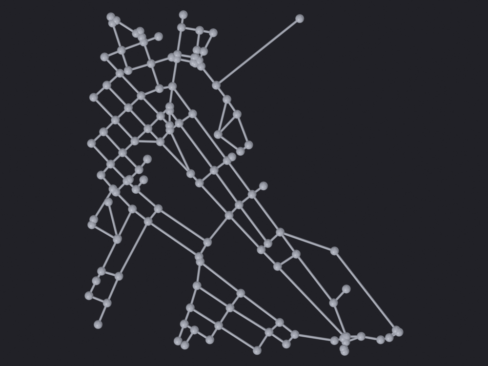
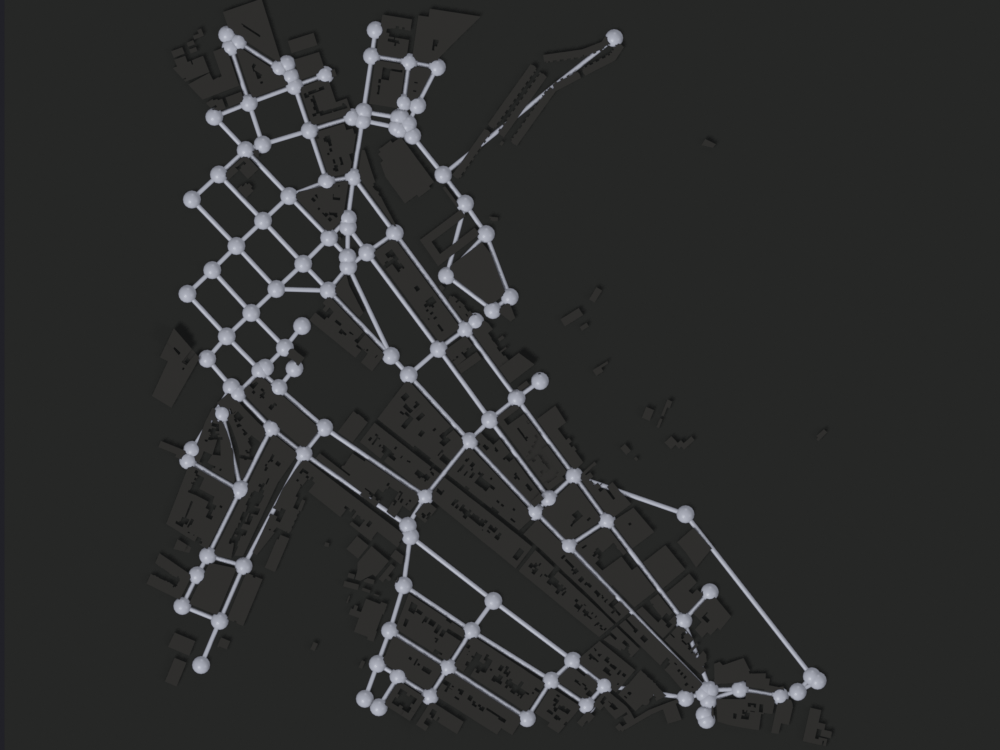
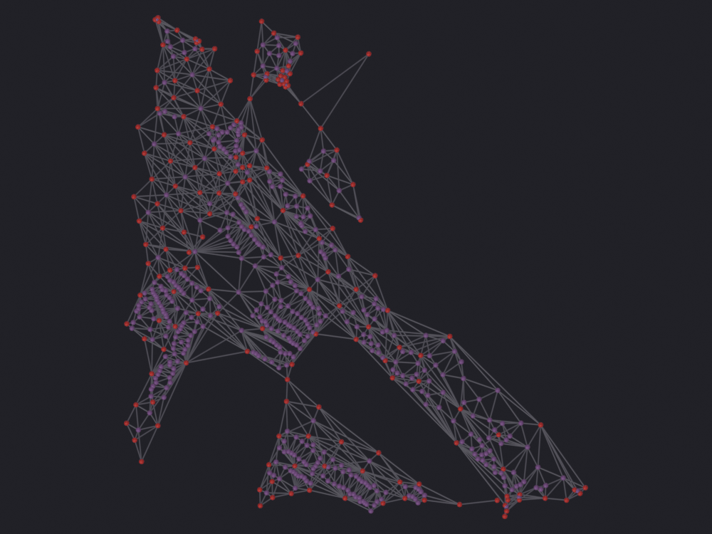
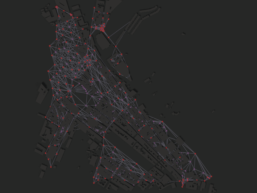
Both of City2Graph’s morphological constructions, each brought into Blender as a native SciGraphs object colored by layer. segments_to_graph() gives the homogeneous primal graph, intersections as nodes and street segments as edges. morphological_graph() gives the heterogeneous graph, where street segments are the channels movement organizes along (public) and plots with their buildings are the units where activity happens (private), stitched together by three relations: (private, touched_to, private), (public, connected_to, public) and (private, faced_to, public).
Input comes from OpenStreetMap via OSMnx rather than from Overture Maps, because Overture reads remote parquet and takes minutes even for one neighborhood; the Overture path is an optional cell at the end. The c2g_generate_tessellation operator passes buildings=/barriers= arguments the API does not have, so they are silently discarded and the tessellation is never enclosed.
13 · Urban morphology
City2Graph has two morphological constructions:
segments_to_graph(): homogeneous primal graph. Intersections are nodes, street segments are edges, street topology and nothing else.
morphological_graph(): heterogeneous graph. Street segments are the channels movement is organized through (public), plots with their buildings are the units where activities take place (private). Three relations stitch it together: (private, touched_to, private) for contiguity between plots, (public, connected_to, public) for street continuity, (private, faced_to, public) for a plot facing the street.
Both become native SciGraphs objects below, colored by layer.
0 · Setup
import pathlibimport sysdef find_repo():"""Locate the SciGraphs repository, without relying on the cwd. In a normal Jupyter the kernel starts per notebook with the cwd set to its folder. Not here: the kernel lives inside Blender and existed before you opened anything, so the cwd is wherever Blender was launched from. What the extension does know is which folder it is serving to JupyterLab. """ candidates = []try:import bpy prefs = bpy.context.preferences.addons["bl_ext.user_default.jupyter_blender"].preferences candidates.append(pathlib.Path(bpy.path.abspath(prefs.notebook_dir)))exceptException:pass candidates.append(pathlib.Path.cwd())for base in candidates:for directory in (base, *base.parents):if (directory /"SciGraphs"/"api"/"graphs.py").is_file():return directoryraiseRuntimeError("Cannot find the SciGraphs repository. Point at it by hand:\n"" sys.path.insert(0, '/path/to/SciGraphs-1/notebooks/tools')")sys.path.insert(0, str(find_repo() /"notebooks"/"tools"))import bpyimport city2graph as c2gimport geopandas as gpd# `nb` must import first: it puts this repository on sys.path, so the# `SciGraphs` import below reads this tree, not the copy Blender installed.import nbfrom nb import checkfrom SciGraphs import api as sgox = nb.osmnx()# A small radius keeps this to seconds; tessellation is the expensive part.CENTER = (39.5093, -0.4084) # Burjassot, ValenciaRADIUS_M =500METRIC_CRS ="EPSG:25830"# UTM 30Nprint("city2graph", c2g.__version__, "| osmnx", ox.__version__)
city2graph 0.3.1 | osmnx 2.0.7
1 · Input data
OpenStreetMap via OSMnx, which answers in seconds. Overture Maps, the other source city2graph supports natively, is the optional cell at the end.
That MultiIndex (from_private_id, to_private_id), whatever it is called in a given construction, is what SciGraphs uses to resolve which vertices an edge joins. An edge GeoDataFrame with a flat index produces an object with vertices and zero edges.
check("the edges carry a MultiIndex (source, target)", edges_primal.index.nlevels >=2,f"levels: {edges_primal.index.nlevels}")
[PASS] the edges carry a MultiIndex (source, target) — levels: 2
True
Into Blender
sg.graphs.anchor_from() creates the georeference object SciGraphs needs to project. Without it create_native_graph_from_gdfs returns None without saying anything. An OSMnx import from the panel leaves one behind; from a bare GeoDataFrame you have to put it there.
sg.graphs.clear_scene(keep_anchor=False)anchor = sg.graphs.anchor(CENTER[0], CENTER[1], scale=0.001, name="Anchor_Morphology")obj_primal = sg.graphs.from_gdf( nodes_primal, edges_primal, name="Primal_Streets", ref=anchor, coll="C2G_Morphology", markers={"graph_type": "segments_to_graph"})print(sg.graphs.summary(obj_primal))check("the primal graph is in the scene", obj_primal isnotNone)check("it has mesh edges", obj_primal isnotNoneandlen(obj_primal.data.edges) >0)
{'object': 'Primal_Streets', 'type': 'MESH', 'num_nodes': 127, 'num_edges': 179, 'is_directed': False, 'vertices': 127, 'mesh_edges': 179, 'attributes': ['position', '.edge_verts', '.corner_vert', '.corner_edge', 'node_id'], 'graph_type': 'segments_to_graph'}
[PASS] the primal graph is in the scene
[PASS] it has mesh edges
True
How the figures in these notebooks are made
The images come from EEVEE, not from the add-on’s own engine. scene.render.engine = 'SCIGRAPHS' rasterizes the GPU buffers of the interactive preview: fast and faithful to the viewport, but it draws graphs and nothing else, with no materials, shadows or ground. nb.figure() switches the add-on onto its other display path (scigraphs_display_engine = 'GEOMETRY_NODES', a modifier instancing spheres on the vertices and sweeping tubes along the edges), so the graph becomes ordinary meshes that lights and shadows act on. sg.context.add_context() fills that scene: a ground surface, and the OSM footprints extruded through the same anchor as the graph and dropped to street level under it. The prisms are display geometry; nothing downstream reads them.
isolate= defaults to True and hides every other mesh, which is wrong when the context is the point, so every context render below passes isolate=False.
Every figure here is straight down through an orthographic camera (render_eevee’s default view='TOP') with look='ink', so what separates them is the attribute they are colored by: here layer_id. The primal graph is the exception, since segments_to_graph() gets geometry and only geometry, so its mesh carries no scalar attribute and it renders in the look’s neutral.
print("attributes on the primal graph:")for name, domain, dtype in sg.graphs.attributes(obj_primal):print(f" {name:<28}{domain:<7}{dtype}")nb.figure(obj_primal, "renders/09_morphology/1_primal", look='ink')
attributes on the primal graph:
  position                     POINT   FLOAT_VECTOR
  .edge_verts                  EDGE    INT32_2D
  .corner_vert                 CORNER  INT
  .corner_edge                 CORNER  INT
  node_id                      POINT   INT
Info: Geometry Nodes modifier added
[PASS] 1_primal.png legible — 8.4% ink (healthy range 0.5–60%)
3 · Tessellation: create_tessellation()
The heterogeneous graph needs the buildings turned into a system of plots, and city2graph wraps momepy’s morphological tessellation for it.
primary_barriers is the parameter that matters: with it the tessellation is enclosed by the street network, each cell belonging to a block; without it the cells cross the streets. The enclosed one is what a plot system needs.
# n_jobs=1 because the default -1 has momepy fork through joblib/loky, and the# children do not inherit the add-on's sys.path inside Blender: every one dies# with `ModuleNotFoundError: No module named 'joblib'`. It still finishes, but# under a wall of tracebacks.cells = c2g.create_tessellation( buildings_m, primary_barriers=segments, shrink=0.4, segment=0.5, n_jobs=1,)print(f"tessellation cells: {len(cells)}")print("columns:", list(cells.columns))cells.head(3)
The same tessellation without barriers, for comparison:
cells_no_barriers = c2g.create_tessellation(buildings_m, shrink=0.4, segment=0.5, n_jobs=1)print(f"with barriers : {len(cells)} cells, mean area {cells.area.mean():.0f} m2")print(f"without barriers: {len(cells_no_barriers)} cells, "f"mean area {cells_no_barriers.area.mean():.0f} m2")check("the barriers change the result",abs(cells.area.mean() - cells_no_barriers.area.mean()) >1.0,"if the areas match, the barriers are being ignored")
with barriers   : 475 cells, mean area 654 m2
without barriers: 1023 cells, mean area 1010 m2
[PASS] the barriers change the result — if the areas match, the barriers are being ignored
True
Warning about the equivalent SciGraphs operator.bpy.ops.scigraphs.c2g_generate_tessellation() calls create_tessellation(geometry=..., buildings=..., barriers=...), and buildings and barriers do not exist in the city2graph 0.3.1 API: **kwargs absorbs them and they are discarded without error. The result is always pure morphological tessellation, whatever you select as barriers in the panel. The correct name is primary_barriers; until the operator is fixed, use the direct call above.
The cells, in Blender
This is not a graph, it is background geometry: polygons as faces.
Using reference projection: center=(39.509300, -0.408400), scale=0.001
Created 1 object(s) from GeoDataFrame with 475 features
Using reference projection: center=(39.509300, -0.408400), scale=0.001
Created 1 object(s) from GeoDataFrame with 1023 features
  Tessellation               9872 vertices,   477 faces
  Buildings                  8154 vertices,  1070 faces
The same buildings, as context under the graph
The SciGraphs engine draws graphs, and a tessellation is a polygon soup with no nodes and no edges, so rendering these two objects through it gives an empty frame. EEVEE has no such restriction, and the useful picture is the street graph standing on the fabric it abstracts.
Three arguments deserve a note:
buildings_gdf=buildings passes the untrimmed download, still carrying its OSM tags. buildings_m keeps only geometry, so a skyline built from it falls back to a constant. Read the tagged fraction the call prints before believing any height.
terrain_source="flat" builds a plane and touches no network. Burjassot has a few meters of relief across the whole frame, not enough to see; notebook 17 fetches a real DEM where it is.
The context radius is larger than the study radius. The camera is orthographic and framed tight on the graph, and the frame is 4:3 while a terrain is square, so ground built at exactly the graph’s radius leaves a strip of bare backdrop down each side, and not a symmetric one, since the graph is not centered on the anchor the way the terrain is. Half as much ground again costs nothing, the plane being generated rather than downloaded, and buildings_gdf was fetched at RADIUS_M, so a wider clip invents no footprints. Worth copying into every context render in the series.
# Same footprints at the graph's exact z. Coplanar surfaces z-fight, so these# step out for the render.for obj in objs_cells + objs_buildings: obj.hide_render =Truectx = sg.context.add_context(obj_primal, CENTER, RADIUS_M *1.5, anchor, buildings_gdf=buildings, terrain_source="flat")print("real elevation:", ctx["real_elevation"])sg.context.report(ctx["objects"])
Creating terrain mesh: 2x2 vertices
Terrain mesh created: 4 vertices, 1 faces
  flat ground, 1500 x 1500 m (no elevation data)
  1023 footprints -> 9224 faces, 16308 vertices
  heights: 15 from OSM tags (1.5%), the rest at 9.0 m (fallback constant)
  context moved -0.00100 Blender units (-1.0 m) so the ground clears z=0 by 1 m
[PASS] Context_Ground aligned with Primal_Streets — center off by 0.0423 BU (3.07% of the graph diagonal), covers 100.0% of it, 1.61x its width
[PASS] Context_Buildings aligned with Primal_Streets — center off by 0.0157 BU (1.14% of the graph diagonal), covers 100.0% of it, 1.05x its width
real elevation: False
  Context_Ground         ground     1.500 x 1.500 x 0.000 BU   source=flat real_elevation=False imagery=none
  Context_Buildings      buildings  0.979 x 1.068 x 0.018 BU   1023 footprints, 1% tagged, default 9.0 m (fallback constant)
Turning the context down
An adjustment the composites here need and the ones in 03 do not. It is a property of the attribute, not of the look.
sg.context’s palette was set against a light backdrop. On this frame it puts the roofs at luminance 101 out of 255 and the ground at 65, where notebook 15’s zone plates land too, so the palette is not the odd one out. The graph on top is what differs. In 03 the colormap is on the edges and takes mid-ramp values, so the network reaches 146 to 202, 45 levels clear of its context. Here it is on the nodes, and layer_id has exactly two values, so it uses turbo’s two endpoints, both of them its darkest stops: private nodes at 90, public at 61, below the roofs at 101. At normal viewing size the layer split stops being visible at all.
61 is what turbo’s top stop is worth under this rig, so the fabric comes down instead. The albedos below put the roofs at 47 and the ground at 39 against a backdrop of 33: an 8-level step, thin but readable because the prisms cast shadows and catch the key at varying angles. The cost is that the buildings read as texture rather than as the subject. The dimming goes in before the first composite rather than between the two, so both composites of the same place are made of the same material.
# Base colors only; the rest of `sg.context.material()` is left alone.CONTEXT_ALBEDO = {"buildings": (0.033, 0.032, 0.029),"terrain": (0.023, 0.024, 0.020),"ground": (0.023, 0.024, 0.022)}def dim_context(objects):"""Scale the context materials down so the graph is the brightest thing.""" done = {}for obj in objects: kind = obj.get("scigraphs_context_kind") or"ground"for mat in obj.data.materials:if mat isNoneor mat.name in done:continue node =next((n for n in mat.node_tree.nodesif n.type=='BSDF_PRINCIPLED'), None)if node isNoneor"Base Color"notin node.inputs:continue rgb = CONTEXT_ALBEDO.get(kind, CONTEXT_ALBEDO["ground"]) node.inputs["Base Color"].default_value = (*rgb, 1.0) mat.diffuse_color = (*rgb, 1.0) done[mat.name] = (kind, rgb)return donefor name, (kind, rgb) in dim_context(ctx["objects"]).items():print(f" {name:<26}{kind:<10} albedo {rgb}")
No satellite imagery under this one, although add_context() will drape it and notebooks 16 and 17 use it. The footprints are already in the frame as prisms, and a photograph of the same roofs would draw them a second time.
# Why every overhead context render here lifts `check_render`'s 60 % ink cap,# explained once. `nb.ink()` counts pixels differing from the top-left pixel,# which over full-frame ground is whatever the corner happens to land on: a# sliver of backdrop there scores the figure 99.6 %, ground reaching the corner# scores the same figure 24 %. A 0.99 ceiling would just fire on corner luck,# so it is removed. The floor still catches an empty render, which scores 0.path = nb.render(obj_primal, "renders/09_morphology/2_primal_context", isolate=False, look='ink', verbose=False)nb.show(path)nb.check_render(path, maximum=1.0)
Info: Geometry Nodes modifier added
[PASS] 2_primal_context.png legible — 21.7% ink (healthy range 0.5–100%)
True
4 · Morphological graph: morphological_graph()
The central construction of the module. Returns (nodes_dict, edges_dict):
nodes_dict has the keys "private" (tessellation cells) and "public" (street segments).
edges_dict is indexed by triplets(source_type, relation, target_type), city2graph’s convention for heterogeneous graphs.
clipping_buffer clips around center_point to distance meters, left generous so as not to lose any of the requested area.
nodes
  private                    1616 Point
  public                      179 Point
edges
  private -> touched_to -> private                        870
  public -> connected_to -> public                        375
  private -> faced_to -> public                           974
[PASS] relation ('private', 'touched_to', 'private') — 870 edges
[PASS] relation ('public', 'connected_to', 'public') — 375 edges
[PASS] relation ('private', 'faced_to', 'public') — 974 edges
The heterograph, in Blender
All the layers land in a single mesh. Each vertex carries a layer_id and each edge an edge_type_id, both integers, so the SciGraphs coloring pipeline can pull the layers apart again.
obj_morpho = sg.graphs.from_hetero( nodes_dict, edges_dict, name="Morphological_Graph", ref=anchor, coll="C2G_Morphology", markers={"graph_type": "morphological_graph"})print(sg.graphs.summary(obj_morpho))print("\nattributes available for coloring:")for name, domain, dtype in sg.graphs.attributes(obj_morpho):print(f" {name:<28}{domain:<7}{dtype}")check("the heterograph is in the scene", obj_morpho isnotNone)
{'object': 'Morphological_Graph', 'type': 'MESH', 'num_nodes': 1795, 'num_edges': 2219, 'is_directed': False, 'vertices': 1795, 'mesh_edges': 2219, 'attributes': ['position', '.edge_verts', '.corner_vert', '.corner_edge', 'layer_id', 'node_id', 'node_enclosure_index', 'edge_type_id', 'edge_weight', 'edge_enclosure_index'], 'layer_names': 'private,public', 'edge_type_names': 'private_touched_to_private,public_connected_to_public,private_faced_to_public', 'graph_type': 'morphological_graph'}

attributes available for coloring:
  position                     POINT   FLOAT_VECTOR
  .edge_verts                  EDGE    INT32_2D
  .corner_vert                 CORNER  INT
  .corner_edge                 CORNER  INT
  layer_id                     POINT   INT
  node_id                      POINT   INT
  node_enclosure_index         POINT   FLOAT
  edge_type_id                 EDGE    INT
  edge_weight                  EDGE    FLOAT
  edge_enclosure_index         EDGE    FLOAT
[PASS] the heterograph is in the scene
True
layer_id is the attribute worth coloring by, and the construction produced it. Two values, two ends of turbo: private (tessellation cells) dark blue, public (street segments) red.
It is on the POINT domain, so the colormap lands on the node spheres and the tubes take the look’s edge_color, a neutral. That neutral has to sit below both node colors, and ink’s default does not, because turbo’s endpoints are the darkest stops on the ramp. It is set explicitly below, to the same value in both figures, so the isolated graph and the composite are one drawing.
print("layer_id domain:", sg.render.attribute_domain(obj_morpho, "layer_id"))# Turbo's endpoints cap the node spheres at luminance 84, so brighter tubes# bury the color. Ink's own 0.13 puts them at 89 and the violet private nodes# dissolve; 0.19 reaches 118, and the 0.50 graph neutral gives a white web with# dark beads. 0.085 lands at 75, under both node classes and still 28 levels# clear of the dimmed roofs.LAYER_EDGE_COLOR = (0.085, 0.080, 0.100)nb.figure(obj_morpho, "renders/09_morphology/3_morphological", look='ink', color_attribute="layer_id", edge_color=LAYER_EDGE_COLOR)
layer_id domain: POINT
  Promoted 3 edge attribute(s) to point domain for GN propagation
Info: Geometry Nodes modifier added
Info: Attribute -> layer_id  ·  layer_id -> turbo [log]  [0 … 1] on Point
[PASS] 3_morphological.png legible — 14.7% ink (healthy range 0.5–60%)
The same graph over the buildings, the picture the whole notebook is for: the private nodes are the tessellation cells wrapped around those prisms.
settle() puts the ground one meter below the plane the graph is drawn on, not below the roofs, so the network is at street level and the taller buildings rise through it. Straight down that shows as a roof occluding the edge behind it. That is a building, not an artifact.
# The 0.35 default is calibrated from the graph's median nearest-neighbor# distance, and this graph interleaves cell and segment layers, so 0.35 draws# spheres the size of a city block. Turbo's dark endpoints mean area is the# only term left: 0.14 gave the colored part 1038 pixels, 0.30 gives 7300.## The primal graph from section 2 hides because `isolate=False` would render it# too, at its own larger `node_fraction`, over the same intersections.if obj_primal isnotNone: obj_primal.hide_render =Truepath = nb.render(obj_morpho,"renders/09_morphology/4_morphological_context", isolate=False, look='ink', color_attribute="layer_id", edge_color=LAYER_EDGE_COLOR, node_fraction=0.30, verbose=False)nb.show(path)nb.check_render(path, maximum=1.0)if obj_primal isnotNone: obj_primal.hide_render =False
  Promoted 3 edge attribute(s) to point domain for GN propagation
Info: Geometry Nodes modifier added
Info: Attribute -> layer_id  ·  layer_id -> turbo [log]  [0 … 1] on Point
[PASS] 4_morphological_context.png legible — 10.6% ink (healthy range 0.5–100%)
5 · Visualize
Without the Geometry Nodes tree that setup_visualization() builds, the graph is a wireframe: correct, but nearly invisible.
sg.graphs.visualize(obj_morpho, node_size=0.02, edge_thickness=0.004)sg.graphs.color_by(obj_morpho, "layer_id", colormap="viridis")sg.graphs.frame(obj_morpho)print("Look at the Blender window: blue = plots (private), ""yellow = street segments (public).")
  Promoted 3 edge attribute(s) to point domain for GN propagation
Info: Geometry Nodes modifier added
Info: Attribute -> layer_id  ·  layer_id -> viridis [log]  [0 … 1] on Point
Look at the Blender window: blue = plots (private), yellow = street segments (public).
6 · What can be measured on this
The SciGraphs analysis operators act on this graph as on any other. On the city2graph side, the heterograph converts to NetworkX losslessly, both ways.
G_hetero = c2g.gdf_to_nx(nodes=nodes_dict, edges=edges_dict)print(f"NetworkX: {G_hetero.number_of_nodes()} nodes, "f"{G_hetero.number_of_edges()} edges")nodes_back, edges_back = c2g.nx_to_gdf(G_hetero, nodes=True, edges=True)total_out =sum(len(v) for v in nodes_dict.values())total_back =sum(len(v) for v in nodes_back.values()) ifisinstance(nodes_back, dict) elselen(nodes_back)check("gdf -> nx -> gdf preserves the node count", total_out == total_back, f"{total_out} vs {total_back}")
NetworkX: 1795 nodes, 2219 edges
[PASS] gdf -> nx -> gdf preserves the node count — 1795 vs 1795
written to notebooks/out/13_morphology
   private.gpkg 2175 kB
   public.gpkg 139 kB
   tessellation.gpkg 356 kB
8 · Optional: the same morphology from Overture Maps
load_overture_data() reads remote GeoParquet: several minutes for a neighborhood, tens of them for a city. Set RUN_OVERTURE = True when you have the time.
Do not skip process_overture_segments(). It splits the segments at the connectors, groups endpoints with slightly different coordinates and reads the metadata to flag impassable segments. It also creates the barrier_geometry column that morphological_graph() looks for in primary_barrier_col.
RUN_OVERTURE =Falseif RUN_OVERTURE:import math lat, lon = CENTER degrees = RADIUS_M /111_000.0 bbox = [lon - degrees / math.cos(math.radians(lat)), lat - degrees, lon + degrees / math.cos(math.radians(lat)), lat + degrees] data = c2g.load_overture_data( bbox, types=["building", "segment", "connector"], save_to_file=False, return_data=True)print({k: len(v) for k, v in data.items()}) seg_ov = c2g.process_overture_segments( data["segment"].to_crs(METRIC_CRS), connectors_gdf=data["connector"].to_crs(METRIC_CRS), get_barriers=True) nodes_ov, edges_ov = c2g.morphological_graph( buildings_gdf=data["building"].to_crs(METRIC_CRS), segments_gdf=seg_ov, center_point=center_m, distance=RADIUS_M, clipping_buffer=100.0) nb.describe_hetero(nodes_ov, edges_ov) sg.graphs.from_hetero(nodes_ov, edges_ov, name="Morphological_Graph_Overture", ref=anchor, coll="C2G_Morphology_Overture")else:print("Overture disabled. Set RUN_OVERTURE to True to try it.")
Overture disabled. Set RUN_OVERTURE to True to try it.
Rendering, in more detail
nb.render() does four things before firing.
It sizes the Geometry Nodes glyphs. The tree bakes node radius and edge thickness into its primitive nodes at build time and exposes no socket for them, so the sizes are written on the object and the tree rebuilt. The radius comes from the median nearest-neighbor distance. The default 0.02 Blender units suits an abstract graph about ten units across; a neighborhood at scale=0.001 measures about one.
It frames the camera with camera_fit_coords against the render aspect, so the resolution is set first. Straight down and orthographic, both by default: a vertical edge at the corner of the frame splays 14.4 px under perspective and 39.0 px from an oblique angle, against 0.0 px here, and on a map that lean is read as geometry. view='OBLIQUE' is for figures about relief or height.
It lights the scene with three suns. A sun’s strength is an irradiance and does not fall off with distance, so one rig is correctly exposed at scale=0.001 and at 1:1. A Light Path node shows the world one color to the camera and a brighter one to the surfaces, so the backdrop stays near-black without the unlit side of every node sphere going with it.
And it checks legibility from the fraction of pixels carrying ink: above 60 % the nodes have merged into a blob, below 0.5 % there is nothing to see. That ceiling assumes an empty field, so the overhead context views raise it.
color_attribute= colors on the freshly rebuilt tree, so the mapping survives the rebuild. look= picks one of five backdrop/palette pairs, each naming a colormap measured to stay clear of its own backdrop at both ends; notebooks 00 to 07 all pass 'ink'. The view transform is Standard, not AgX, which rolls off highlights and desaturates. The PNGs land in notebooks/out/renders/.
Applies to the SciGraphs engine, not to EEVEE: on Blender’s Vulkan backend, the default on Linux, gpu.state.point_size_set does nothing for the add-on’s shaders, so POINT and DISK nodes come out 1 pixel wide. Start Blender with --gpu-backend opengl for any render you intend to look at.
Summary
Step
city2graph function
Result in Blender
Primal graph
segments_to_graph()
Primal_Streets
Plots
create_tessellation(primary_barriers=…)
Tessellation
Heterogeneous graph
morphological_graph()
Morphological_Graph
Next: 02 · Transport (GTFS).
print("Objects in the scene:")for obj in bpy.data.objects:print(f" {obj.name:<32}{obj.type}")
Objects in the scene:
  Anchor_Morphology                EMPTY
  Buildings                        MESH
  Context_Buildings                MESH
  Context_Ground                   MESH
  Morphological_Graph              MESH
  Primal_Streets                   MESH
  SciGraphs_Camera                 CAMERA
  SciGraphs_Fill                   LIGHT
  SciGraphs_Key                    LIGHT
  SciGraphs_Rim                    LIGHT
  Tessellation                     MESH