import importlib
import math
import pathlib
import sys
import time


def find_repo():
    """Locate the SciGraphs repository, without relying on the cwd.

    In a normal Jupyter the kernel starts per notebook with the cwd set to its
    folder. Not here: the kernel lives inside Blender and existed before you
    opened anything, so the cwd is wherever Blender was launched from. What the
    extension does know is which folder it is serving to JupyterLab.
    """
    candidates = []
    try:
        import bpy
        prefs = bpy.context.preferences.addons[
            "bl_ext.user_default.jupyter_blender"].preferences
        candidates.append(pathlib.Path(bpy.path.abspath(prefs.notebook_dir)))
    except Exception:
        pass
    candidates.append(pathlib.Path.cwd())

    for base in candidates:
        for directory in (base, *base.parents):
            if (directory / "SciGraphs" / "api" / "graphs.py").is_file():
                return directory

    raise RuntimeError(
        "Cannot find the SciGraphs repository. Point at it by hand:\n"
        "    sys.path.insert(0, '/path/to/SciGraphs-1/notebooks/tools')")


sys.path.insert(0, str(find_repo() / "notebooks" / "tools"))

import bpy
import geopandas as gpd
import networkx as nx
import numpy as np

# `nb` must import first: it puts this repository on sys.path, so the
# `SciGraphs` import below reads this tree, not the copy Blender installed.
import nb
from nb import check

from SciGraphs import api as sg06 · Downloading a street network
Get a street network in, clean it, know what you have. The other four OSMnx notebooks assume it.
The same neighborhood downloaded as drive, bike, walk and all gives 243, 814, 1582 and 1894 intersections, and comparing their lengths naively inflates the walk-to-drive ratio from 2.4× to 4.6×, because summing a directed multigraph double-counts two-way streets and a drive network here is 98 % one-way. Simplification removes 79 % of the nodes without changing a meter of length; consolidation at a 40 m tolerance moves one node 302 m, since a chain of intersections collapses to a point that need not lie near any of its members.
Several operators are wrong, and the notebook says so where it meets them: a bounding box passed in the wrong order silently reduces a 243-node network to 2 while reporting success, a cache key omits the radius so six downloads overwrite one file, and a family of cleaning operators replace the graph and never rebuild the mesh you are looking at.
06 · OSMnx: getting a street network in, and knowing what you have
First of five notebooks that treat the street network as the object of study rather than as scenery under a city2graph result. This one is the download, the cleaning, and the arithmetic that tells you what you got.
Which graph you have is decided by four settings:
- the download method: place, point, address, bounding box, polygon. Five ways of saying “Ciutat Vella, about 600 m”, and five different graphs.
network_type:drive,bike,walkandallgive 243, 814, 1582 and 1894 intersections over the same disc of Valencia.- simplification, which removes four nodes in every five.
- consolidation, which merges what is left, and can merge too much.
None is right or wrong on its own; not knowing which one you took is.
The study area is Ciutat Vella, València (39.4699, -0.3763) on a 600 m radius: a few hundred kilobytes from Overpass rather than a few hundred megabytes.
The next four: edge attributes, speeds and orientation (11), routing and isochrones (12), accessibility and points of interest (13), centrality and export (14). Elevation belongs to 08.
0 · Setup
The cache goes first, before anything downloads
nb.osmnx() sets ox.settings.use_cache and ox.settings.cache_folder. The add-on sets only the first (SciGraphs/core/city2graph/data.py:47), and the osmnx_cache_directory preference defaults to empty, so OSMnx falls back to a relative path resolved against wherever Blender was launched from: run the notebook from two places and you have two caches, neither ever hit twice.
Overpass is a shared public service with a per-IP slot limit. Re-downloading on every run collects an HTTP 429, then Errno 111 Connection refused, then an outright failure that reads like a bug in the code. With the cache, a re-run is offline in fifteen seconds.
Call it before the first operator, not merely before the first ox. call: the importer imports the same osmnx module object this notebook does, so whatever cache_folder says when the operator runs is where it looks.
ox = nb.osmnx()

print(f"osmnx        {ox.__version__}")
print(f"use_cache    {ox.settings.use_cache}")
print(f"cache_folder {nb.rel(ox.settings.cache_folder)}")

CACHE_DIR = pathlib.Path(ox.settings.cache_folder)
responses = sorted(CACHE_DIR.glob("*.json")) if CACHE_DIR.is_dir() else []
print(f"{len(responses)} cached Overpass responses, "
      f"{sum(p.stat().st_size for p in responses) / 1e6:.1f} MB")
osmnx 2.0.7
use_cache True
cache_folder notebooks/data/cache/osmnx
47 cached Overpass responses, 81.5 MBThe study area, and why the modules come from the add-on
The operators run inside the copy of SciGraphs that Blender registered, and the graph they leave behind lives in a module-level dict inside that copy. import SciGraphs reaches a different module object with an empty cache, and every get_osmnx_graph would come back None (notebook 11 has the detail), so everything below reaches for the installed package by name.
CENTER = (39.4699, -0.3763)      # Ciutat Vella, València
RADIUS_M = 600
PLACE = "Ciutat Vella, València, Spain"
ADDRESS = "Plaça de la Reina, València, Spain"

INSTALLED = next(k for k in bpy.context.preferences.addons.keys()
                 if k.rsplit(".", 1)[-1].lower() == "scigraphs")
graph_cache = importlib.import_module(INSTALLED + ".core.osmnx.graph_cache")
# `scigraphs_core` is a wheel: one copy in site-packages, shared by the notebook
# and the operators, so the installed/working-tree split does not apply to it.
convert = importlib.import_module("scigraphs_core.osmnx.convert")
geocoder = importlib.import_module("scigraphs_core.osmnx.geocoder")
mesh_bridge = importlib.import_module("scigraphs_core.osmnx.mesh_bridge")
sg_cache = importlib.import_module(INSTALLED + ".core.osmnx.cache")
sg_importer = importlib.import_module(INSTALLED + ".core.data_io.importer")
sg_geometry = importlib.import_module(INSTALLED + ".core.mesh.geometry")

print("add-on package :", INSTALLED)
print("graphml cache  :", nb.rel(sg_cache.get_cache_directory()))
add-on package : bl_ext.user_default.scigraphs
graphml cache : ~/.config/blender/5.2/scripts/addons/scigraphs_osmnx_cacheFour helpers, and why each has to exist
download(...) fires scigraphs.import_osm_graph. The operator reads all the OSMnx properties off scene.scigraphs, so a property left set by an earlier cell is the easiest way to get a graph you did not ask for. This resets the lot, every time.
materialize(G, name) builds a Blender object from a NetworkX graph. The cleaning operators replace the graph in the in-memory cache and nowhere else and leave the mesh at its old node and edge counts (section 3), so rebuilding is the only way to draw what they produced.
node_attribute(...) puts a per-node quantity on the mesh so a figure can be colored by it. mesh_bridge.transfer_node_attribute_to_mesh does the first half only. An OSMnx mesh has many more vertices than nodes, because retain_geometry stores the shape of every street as intermediate points, and that function leaves every one at 0.0: they get no node glyph but they do land in the attribute’s range, so the color scale starts at a value no intersection has. Here each takes the mean of the two intersections its street runs between, the convention Blender uses when averaging edge attributes onto points.
counts(G) prints three numbers the same way every time, so fifteen graphs can be compared down a column.
def download(method='POINT', network_type='drive', simplify=True,
             retain_all=False, truncate_by_edge=True, place='', address='',
             bbox=None, distance=RADIUS_M, center=CENTER, polygon_object=''):
    """Set every OSMnx scene property, then run `scigraphs.import_osm_graph`.

    `bbox` is `(west, south, east, north)`, the order OSMnx 2.x uses
    everywhere and the order section 1 shows the add-on's own helper does not.
    Returns the new object, or None when the download failed.
    """
    props = bpy.context.scene.scigraphs
    props.osmnx_download_method = method
    props.osmnx_network_type = network_type
    props.osmnx_simplify = bool(simplify)
    props.osmnx_retain_all = bool(retain_all)
    props.osmnx_truncate_by_edge = bool(truncate_by_edge)
    props.osmnx_retain_geometry = True
    props.osmnx_custom_filter_preset = 'NONE'
    props.osmnx_custom_filter_text = ""
    props.osmnx_which_result = 0
    props.osmnx_scale = 0.001
    props.osmnx_place_name = place
    props.osmnx_address = address
    props.osmnx_polygon_object = polygon_object
    props.osmnx_latitude, props.osmnx_longitude = center
    props.osmnx_distance = int(distance)
    if bbox is not None:
        (props.osmnx_bbox_west, props.osmnx_bbox_south,
         props.osmnx_bbox_east, props.osmnx_bbox_north) = bbox

    started = time.time()
    try:
        result = bpy.ops.scigraphs.import_osm_graph()
    except RuntimeError as exc:          # the operator reports and cancels
        print(f"  import_osm_graph failed: {exc}")
        return None
    if 'FINISHED' not in result:
        return None
    obj = bpy.context.active_object
    obj["download_seconds"] = round(time.time() - started, 2)
    return obj


def materialize(G, name, scale=0.001):
    """A Blender object for a NetworkX graph an operator handed back.

    `create_osmnx_graph_object` reads `x`/`y` as longitude and latitude without
    checking (`_convert_osmnx_coords_to_3d` in
              `SciGraphs/core/mesh/geometry.py`), so a projected graph has to go back to
    EPSG:4326 first (section 4).
    """
    graph_data, geometries = sg_importer.osmnx_to_graph_data(
        G, retain_geometry=True)
    if graph_data is None:
        return None
    obj = sg_geometry.create_osmnx_graph_object(
        graph_data, geometries, scale=scale, retain_geometry=True)
    if obj is None:
        return None
    obj.name = name
    graph_cache.store_osmnx_graph(obj, G)
    obj["osmnx_scale"] = scale
    return obj


def node_attribute(obj, values, name):
    """Write a per-node quantity onto the mesh, filling the street geometry.

    `values` maps node id -> number. Returns (intersections written, array).
    """
    mesh = obj.data
    ids = str(obj.get("nodes_data", "")).split(",")
    array = np.zeros(len(mesh.vertices), dtype=np.float64)
    filled = np.zeros(len(mesh.vertices), dtype=bool)
    touched = np.zeros(len(mesh.vertices), dtype=bool)

    def key(text):
        return int(text) if text.lstrip("-").isdigit() else text

    for index, node_id in enumerate(ids):
        if index >= len(array):
            break
        value = values.get(key(node_id))
        if value is not None:
            array[index] = float(value)
            filled[index] = touched[index] = True

    # Shape vertices take the mean of the two intersections they connect.
    edge_verts = np.empty(len(mesh.edges) * 2, dtype=np.int32)
    mesh.edges.foreach_get("vertices", edge_verts)
    edge_verts = edge_verts.reshape(-1, 2)
    for (u, v), indices in mesh_bridge.build_edge_mapping(obj).items():
        a, b = values.get(key(u)), values.get(key(v))
        if a is None or b is None:
            continue
        middle = 0.5 * (float(a) + float(b))
        for edge_index in indices:
            for vertex in edge_verts[edge_index]:
                if not touched[vertex]:
                    array[vertex] = middle
                    touched[vertex] = True

    # Untouched vertices are geometry whose graph edge the mapping missed: a
    # self-loop or a parallel pair. Zero would plant a value no intersection
    # has at the bottom of every color ramp, so use the mean.
    real = array[filled]
    if len(real) and not touched.all():
        array[~touched] = float(real.mean())

    if name in mesh.attributes:
        mesh.attributes.remove(mesh.attributes[name])
    layer = mesh.attributes.new(name=name, type='FLOAT', domain='POINT')
    layer.data.foreach_set("value", array.astype(np.float32).tolist())
    return int(filled.sum()), array


def counts(G, label=""):
    """`(nodes, edges, kilometers)` for a graph, optionally on one printed line."""
    kilometers = sum(float(d.get("length", 0.0))
                     for *_ids, d in G.edges(data=True)) / 1000.0
    if label:
        print(f"  {label:<30} {G.number_of_nodes():>6} nodes "
              f"{G.number_of_edges():>6} edges {kilometers:>8.1f} km")
    return G.number_of_nodes(), G.number_of_edges(), kilometers


sg.graphs.clear_scene(keep_anchor=False)
props = bpy.context.scene.scigraphs
print("scene cleared")
scene cleared1 · Five ways to say where
osmnx_download_method takes seven values. Five describe an area, and they are not interchangeable.
| Method | You give it | Good for | Fails when |
|---|---|---|---|
PLACE |
"Ciutat Vella, València, Spain" |
administrative units: a district, a municipality, a park | the geocoder returns the wrong one of six matches, or a point where you wanted a polygon |
POINT |
a lat/lon and a radius | “this much around here”: unambiguous, reproducible, no geocoder | the interesting area is not a disc |
ADDRESS |
a postal address and a radius | a study centered on a building | the address geocodes to the street rather than the number |
BBOX |
four numbers | matching somebody else’s extent exactly: a raster tile, a published figure | you have to know the four numbers |
POLYGON |
a Blender mesh | a boundary you already have, or one you drew | the mesh vertices are not lon/lat |
The two left over: MULTI_PLACE unions a list of names, and XML reads a local .osm file and touches no network at all, which is what to reach for when Overpass is refusing connections.
PLACE and ADDRESS cost two round trips: Nominatim to resolve the name, then Overpass for the data, and the first can silently give you a different place next month. POINT and BBOX cost one and are deterministic, which is why every reproducible pipeline in this suite is built on POINT.
The coordinates that go over the wire are not the ones you type
props.osmnx_latitude is a Blender FloatProperty, single precision. 39.4699 has no exact 32-bit representation, so ox.graph_from_point receives 39.46989822387695, about twenty centimeters south of where you asked, and -0.3763 becomes -0.37630000710487366.
Two consequences, neither of them reported anywhere.
- The cache misses. OSMnx keys its response cache on a hash of the Overpass query string, which contains the bounding box computed from these numbers, so a cache warmed by calling
ox.graph_from_point(CENTER, …)by hand is one the operator never hits: the notebook downloads on every run while looking as if it caches. - The graph is different. Not merely renumbered: a shifted box crosses different ways, and the counts move.
props.osmnx_latitude, props.osmnx_longitude = CENTER
queried = (props.osmnx_latitude, props.osmnx_longitude)
meters_per_degree = 111320.0

print(f"asked for    {CENTER[0]!r}, {CENTER[1]!r}")
print(f"queried with {queried[0]!r}, {queried[1]!r}")
print(f"offset       {abs(queried[0] - CENTER[0]) * meters_per_degree * 100:.2f} cm "
      f"north-south, "
      f"{abs(queried[1] - CENTER[1]) * meters_per_degree * math.cos(math.radians(CENTER[0])) * 100:.2f} cm "
      f"east-west")

exact = ox.graph_from_point(CENTER, dist=RADIUS_M, network_type='drive',
                            simplify=True, truncate_by_edge=True)
counts(exact, "float64, calling OSMnx by hand")

net = download('POINT', 'drive')
net.name = "Net_point_drive"
G_point = graph_cache.get_osmnx_graph(net)
counts(G_point, "float32, through the operator")

check("the operator's graph is in the scene",
      net is not None and bool(net.get("is_osmnx")))
check("single precision changes the graph, not just the query string",
      exact.number_of_nodes() != G_point.number_of_nodes(),
      f"{exact.number_of_nodes()} vs {G_point.number_of_nodes()} nodes from "
      "the same request typed two ways")
asked for 39.4699, -0.3763
queried with 39.46989822387695, -0.37630000710487366
offset 19.77 cm north-south, 0.06 cm east-west
float64, calling OSMnx by hand 242 nodes 373 edges 31.6 km
Downloading OSM network (POINT)...
Point: (39.46989822387695, -0.37630000710487366), radius: 600m
Download completed in 0.40s
Total import time: 0.43s
Nodes: 243, Edges: 375
Creating OSMnx graph: 243 nodes, 375 edges...
Created 243 intersection vertices
Created 361 street edges in 0.01s
Total OSMnx graph creation time: 0.01s
Graph saved to ~/.config/blender/5.2/scripts/addons/scigraphs_osmnx_cache/39.4699_-0.3763_drive.graphml
Graph cached to: ~/.config/blender/5.2/scripts/addons/scigraphs_osmnx_cache/39.4699_-0.3763_drive.graphml
Info: Downloading network from OpenStreetMap (POINT)...
Info: Graph cached as: 39.4699_-0.3763_drive.graphml
Info: Imported: 243 intersections, 375 street segments, 31.8 km total
float32, through the operator 243 nodes 375 edges 31.8 km
[PASS] the operator's graph is in the scene
[PASS] single precision changes the graph, not just the query string — 242 vs 243 nodes from the same request typed two waysTrueThe fix is to warm the cache through the operator, as every cell below does, and to treat the float32 value as the reproducible identifier for a point download. Notebook 11 makes the same point from the terrain side, where the rounding decides which DEM tile is fetched.
What the imported object carries
The import writes a mesh and a dozen custom properties. Four are load-bearing: nodes_data and edges_data carry any attribute back onto the mesh, and osmnx_center_lat/lon is the projection origin anything placed alongside the graph has to share.
for key in ("num_nodes", "num_edges", "total_length_m", "num_mesh_verts",
            "osmnx_center_lat", "osmnx_center_lon", "osmnx_scale",
            "osmnx_method", "osmnx_network_type", "osmnx_query_name",
            "is_directed"):
    print(f"  {key:<20} {net.get(key)}")
print(f"  {'mesh vertices':<20} {len(net.data.vertices)}")
print(f"  {'mesh edges':<20} {len(net.data.edges)}")
print("  attributes:", [(a.name, a.domain) for a in net.data.attributes
      if not a.name.startswith(".")])
num_nodes 243
num_edges 375
total_length_m 31782.730552268284
num_mesh_verts 1374
osmnx_center_lat 39.46885868888891
osmnx_center_lon -0.3761819053497941
osmnx_scale 0.0010000000474974513
osmnx_method POINT
osmnx_network_type drive
osmnx_query_name 39.4699_-0.3763
is_directed True
mesh vertices 1374
mesh edges 1492
attributes: [('is_intersection', 'POINT'), ('position', 'POINT')]The trap that decides whether a figure is legible.
create_osmnx_graph_objectwritesnodes_data,edges_data,osmnx_center_latand the rest of the native-graph contract, but notnode_positions(SciGraphs/core/mesh/geometry.py:1750).sg.preview.extent, and through it every node radius and every camera fit, falls back to all mesh vertices, which here means every sample along every street centerline. The median nearest-neighbor distance then measures the sampling step of the road geometry rather than the distance between intersections, and the node radius derived from it is several times too small: a two-pixel node and a sub-pixel tube.
sg.render.node_cloud()reads theis_intersectionvertex layer instead, whichcreate_osmnx_graph_objectdoes write. Every figure below goes throughnb.render, which measures throughnode_cloud.
cloud, source = sg.render.node_cloud(net)
_center, _size, _diagonal, median_nn = sg.render.measure(net)[0]
_c, _s, _d, naive_nn = sg.preview.extent(net)
scale = float(net.get("osmnx_scale", 0.001))

print(f"node_positions present   {'node_positions' in net.keys()}")
print(f"node_cloud source        {source}  ({len(cloud)} of "
      f"{len(net.data.vertices)} vertices)")
print(f"median nearest neighbor {median_nn / scale:>6.1f} m  through node_cloud")
print(f"                         {naive_nn / scale:>6.1f} m  over every vertex")
print(f"node radius would be     "
      f"{median_nn * sg.render.NODE_FRACTION / scale:>6.1f} m  vs "
      f"{naive_nn * sg.render.NODE_FRACTION / scale:.1f} m, a factor of "
      f"{median_nn / naive_nn:.1f}")

check("the node cloud is the intersections, not the street geometry",
      source == "is_intersection" and len(cloud) == net.get("num_nodes"))
node_positions present False
node_cloud source is_intersection (243 of 1374 vertices)
median nearest neighbor 35.1 m through node_cloud
6.1 m over every vertex
node radius would be 12.3 m vs 2.1 m, a factor of 5.7
[PASS] the node cloud is the intersections, not the street geometryTrueResolving a name: the two geocoders
osmnx_geocode turns a place name or an address into a lat/lon and writes it straight into osmnx_latitude/osmnx_longitude, which is how a PLACE question becomes a reproducible POINT download. osmnx_geocode_to_gdf fetches the boundary polygon instead, which is what POLYGON wants.
coords = geocoder.geocode(ADDRESS)
print(f"geocode({ADDRESS!r})\n  -> {coords}")

boundary = geocoder.geocode_to_gdf(PLACE)
print(f"\ngeocode_to_gdf({PLACE!r})")
if boundary is not None and len(boundary):
    print(f"  {len(boundary)} feature(s), crs {boundary.crs}, "
          f"{boundary.geometry.iloc[0].geom_type}")
    print(f"  bounds {[round(v, 5) for v in boundary.total_bounds]}")
    print(f"  area   {boundary.to_crs('EPSG:25830').area.sum() / 1e6:.3f} km2")

check("the address geocodes", coords is not None)
check("the place has a boundary polygon",
      boundary is not None and len(boundary) > 0)
Geocoded 'Plaça de la Reina, València, Spain' to (39.474484, -0.3754586)
geocode('Plaça de la Reina, València, Spain')
-> (39.474484, -0.3754586)
Geocoded 'Ciutat Vella, València, Spain' to GeoDataFrame
geocode_to_gdf('Ciutat Vella, València, Spain')
1 feature(s), crs epsg:4326, Polygon
bounds [np.float64(-0.38416), np.float64(39.46712), np.float64(-0.36601), np.float64(39.48214)]
area 1.721 km2
[PASS] the address geocodes
[PASS] the place has a boundary polygonTrueDefect.
osmnx_geocode_to_gdfthrows the GeoDataFrame away (SciGraphs/ui/operators/osmnx/geocoding_operators.py:28-36): it fetches the boundary, reports how many features came back, and returns{'FINISHED'}with nothing written to the scene, to an object, or to disk. The core function is fine (the cell above calls it); the button spends a Nominatim request and produces no result.
osmnx_bbox_from_point, which has two faults stacked
The button that turns a point and a radius into the four BBOX fields writes 90, 90, 180, 180: the maxima of the four properties, and not a box at all. Two independent faults produce that, and only one of them is visible.
The projection fires first. core/osmnx/utils_geo.py:5 gives bbox_from_point a default of project_utm=True, where OSMnx’s own default is False, and the operator does not pass the argument (geocoding_operators.py:79). The wrapper asks for the box in UTM meters, numbers in the hundreds of thousands, and hands them to four FloatProperty fields clamped to ±90 and ±180 degrees. Every one saturates.
The ordering is underneath. ox.utils_geo.bbox_from_point in OSMnx 2.x returns (left, bottom, right, top), that is (west, south, east, north); the operator assigns bbox[0] to osmnx_bbox_north, bbox[1] to south, bbox[2] to east and bbox[3] to west (geocoding_operators.py:87-90), the OSMnx 1.x order. Fix the projection and this takes over: north receives the longitude of the western edge and west the latitude of the northern edge.
The download path is correct: _osmnx_graph_from_bbox switches on the OSMnx major version and reorders (core/data_io/importer.py:542-557). A BBOX download works, unless the four numbers came from the button next to it.
west, south, east, north = ox.utils_geo.bbox_from_point(CENTER, dist=RADIUS_M)
print(f"ox.utils_geo.bbox_from_point            -> (W, S, E, N) = "
      f"({west:.5f}, {south:.5f}, {east:.5f}, {north:.5f})")
projected = ox.utils_geo.bbox_from_point(CENTER, dist=RADIUS_M,
                                         project_utm=True)
print(f"…the same call with project_utm=True    -> "
      f"{tuple(round(v) for v in projected)}  (UTM meters)")

print("\nosmnx_bbox_from_point ->",
      bpy.ops.scigraphs.osmnx_bbox_from_point(
      latitude=CENTER[0], longitude=CENTER[1], distance=float(RADIUS_M)))
wrote = (props.osmnx_bbox_north, props.osmnx_bbox_south,
         props.osmnx_bbox_east, props.osmnx_bbox_west)
print(f"  wrote N={wrote[0]:.5f}  S={wrote[1]:.5f}  "
      f"E={wrote[2]:.5f}  W={wrote[3]:.5f}")
print("  the property limits are ±90 and ±180, so every field saturated")

# The second fault, with the projection out of the way.
would_be = (west, south, east, north)     # what OSMnx 2.x returns
print(f"\nwith project_utm=False, the operator's own mapping would write")
print(f"  N={would_be[0]:.5f}  S={would_be[1]:.5f}  "
      f"E={would_be[2]:.5f}  W={would_be[3]:.5f}")
print(f"  a usable box needs N > S and E > W:  "
      f"N>S {would_be[0] > would_be[1]},  E>W {would_be[2] > would_be[3]}")

check("osmnx_bbox_from_point cannot produce a usable box",
      not (wrote[0] > wrote[1] and wrote[2] > wrote[3]),
      "UTM meters clamped to degree limits; and under that, north and "
      "west are swapped")
check("the ordering fault is real underneath the projection one",
      not (would_be[0] > would_be[1] and would_be[2] > would_be[3]),
      "read the tuple as (W, S, E, N), or call "
      "ox.utils_geo.bbox_from_point directly, as this notebook does")
ox.utils_geo.bbox_from_point -> (W, S, E, N) = (-0.38329, 39.46450, -0.36931, 39.47530)
…the same call with project_utm=True -> (725077, 4371594, 726315, 4372827) (UTM meters)
Created bbox from point with 600.0m radius
Info: BBox created: 600.0m around point
osmnx_bbox_from_point -> {'FINISHED'}
wrote N=90.00000 S=90.00000 E=180.00000 W=180.00000
the property limits are ±90 and ±180, so every field saturated
with project_utm=False, the operator's own mapping would write
N=-0.38329 S=39.46450 E=-0.36931 W=39.47530
a usable box needs N > S and E > W: N>S False, E>W False
[PASS] osmnx_bbox_from_point cannot produce a usable box — UTM meters clamped to degree limits; and under that, north and west are swapped
[PASS] the ordering fault is real underneath the projection one — read the tuple as (W, S, E, N), or call ox.utils_geo.bbox_from_point directly, as this notebook doesTrueA boundary as a Blender mesh, for POLYGON
The POLYGON method reads a mesh object’s vertex coordinates as longitude and latitude: no transform, no CRS, no check (data_operators.py:562-573). It takes the first face if there is one and all the vertices otherwise, so the boundary from geocode_to_gdf becomes a download boundary by being written into a mesh.
Two details that are not advertised. The polygon is simplified first, to eleven points, because Overpass builds one clause per vertex and a 400-vertex administrative boundary takes minutes and is rejected under load. And mesh coordinates are float32, so the boundary is quantized to about a centimeter on the way in.
outline = boundary.geometry.iloc[0]
if outline.geom_type == 'MultiPolygon':
    outline = max(outline.geoms, key=lambda g: g.area)
ring = list(outline.simplify(0.0004).exterior.coords)[:-1]

aoi_mesh = bpy.data.meshes.new("AOI_Mesh")
aoi_mesh.from_pydata([(x, y, 0.0) for x, y in ring], [],
                     [list(range(len(ring)))])
aoi_mesh.update()
aoi = bpy.data.objects.new("AOI_CiutatVella", aoi_mesh)
bpy.context.scene.collection.objects.link(aoi)
aoi.hide_render = True

print(f"boundary       {len(outline.exterior.coords)} points")
print(f"simplified to  {len(ring)} points, which is {len(ring)} Overpass clauses")
print(f"as float32     {tuple(round(v, 6) for v in aoi_mesh.vertices[0].co[:2])} "
      f"vs {tuple(round(v, 6) for v in ring[0])}")
boundary 159 points
simplified to 11 points, which is 11 Overpass clauses
as float32 (-0.384156, 39.475712) vs (-0.384156, 39.47571)Five methods, five graphs
The same neighborhood asked for five ways, network_type='drive' throughout. All five are recognizably Ciutat Vella.
methods = {}
methods['POINT'] = net
methods['PLACE'] = download('PLACE', place=PLACE)
methods['ADDRESS'] = download('ADDRESS', address=ADDRESS)
methods['BBOX'] = download('BBOX', bbox=(west, south, east, north))
methods['POLYGON'] = download('POLYGON', polygon_object=aoi.name)

print(f"  {'method':<30} {'nodes':>6}       {'edges':>6}       {'km':>8}")
for name, obj in list(methods.items()):
    if obj is None:
        print(f"  {name:<30} download failed: Overpass is refusing "
              "connections; wait and re-run")
        methods.pop(name)
        continue
    obj.name = f"Net_{name.lower()}"
    counts(graph_cache.get_osmnx_graph(obj), name)

check("all five ways of saying where came back",
      len(methods) == 5, f"{sorted(methods)}")
check("no two of them are the same graph",
      len({obj.get("num_nodes") for obj in methods.values()})
      == len(methods),
      "same place, five extents")
Downloading OSM network (PLACE)...
  Place: Ciutat Vella, València, Spain
  Download completed in 0.30s
Total import time: 0.33s
  Nodes: 236, Edges: 358

Creating OSMnx graph: 236 nodes, 358 edges...
  Created 236 intersection vertices
  Created 336 street edges in 0.01s
Total OSMnx graph creation time: 0.01s
Graph saved to ~/.config/blender/5.2/scripts/addons/scigraphs_osmnx_cache/Ciutat_Vella_València_Spain_drive.graphml
Graph cached to: ~/.config/blender/5.2/scripts/addons/scigraphs_osmnx_cache/Ciutat_Vella_València_Spain_drive.graphml
Info: Downloading network from OpenStreetMap (PLACE)...
Info: Graph cached as: Ciutat_Vella_València_Spain_drive.graphml
Info: Imported: 236 intersections, 358 street segments, 33.2 km total

Downloading OSM network (ADDRESS)...
  Address: Plaça de la Reina, València, Spain, radius: 600m
  Download completed in 0.30s
Total import time: 0.32s
  Nodes: 177, Edges: 264

Creating OSMnx graph: 177 nodes, 264 edges...
  Created 177 intersection vertices
  Created 246 street edges in 0.01s
Total OSMnx graph creation time: 0.01s
Graph saved to ~/.config/blender/5.2/scripts/addons/scigraphs_osmnx_cache/Plaça_de_la_Reina_València_Spain_drive.graphml
Graph cached to: ~/.config/blender/5.2/scripts/addons/scigraphs_osmnx_cache/Plaça_de_la_Reina_València_Spain_drive.graphml
Info: Downloading network from OpenStreetMap (ADDRESS)...
Info: Graph cached as: Plaça_de_la_Reina_València_Spain_drive.graphml
Info: Imported: 177 intersections, 264 street segments, 25.1 km total

Downloading OSM network (BBOX)...
  Bounding box: N=39.47529602050781, S=39.46450424194336, E=-0.36931008100509644, W=-0.3832899034023285
  Download completed in 0.41s
Total import time: 0.44s
  Nodes: 242, Edges: 373

Creating OSMnx graph: 242 nodes, 373 edges...
  Created 242 intersection vertices
  Created 359 street edges in 0.01s
Total OSMnx graph creation time: 0.01s
Graph saved to ~/.config/blender/5.2/scripts/addons/scigraphs_osmnx_cache/bbox_39.48_39.46_drive.graphml
Graph cached to: ~/.config/blender/5.2/scripts/addons/scigraphs_osmnx_cache/bbox_39.48_39.46_drive.graphml
Info: Downloading network from OpenStreetMap (BBOX)...
Info: Graph cached as: bbox_39.48_39.46_drive.graphml
Info: Imported: 242 intersections, 373 street segments, 31.6 km total

Downloading OSM network (POLYGON)...
  Polygon: (-0.38415640592575073, 39.46715545654297, -0.36601150035858154, 39.4820671081543)
  Download completed in 0.30s
Total import time: 0.32s
  Nodes: 197, Edges: 298

Creating OSMnx graph: 197 nodes, 298 edges...
  Created 197 intersection vertices
  Created 276 street edges in 0.01s
Total OSMnx graph creation time: 0.01s
Graph saved to ~/.config/blender/5.2/scripts/addons/scigraphs_osmnx_cache/polygon_AOI_CiutatVella_drive.graphml
Graph cached to: ~/.config/blender/5.2/scripts/addons/scigraphs_osmnx_cache/polygon_AOI_CiutatVella_drive.graphml
Info: Downloading network from OpenStreetMap (POLYGON)...
Info: Graph cached as: polygon_AOI_CiutatVella_drive.graphml
Info: Imported: 197 intersections, 298 street segments, 26.7 km total
  method                          nodes        edges             km
  POINT                             243 nodes    375 edges     31.8 km
  PLACE                             236 nodes    358 edges     33.2 km
  ADDRESS                           177 nodes    264 edges     25.1 km
  BBOX                              242 nodes    373 edges     31.6 km
  POLYGON                           197 nodes    298 edges     26.7 km
[PASS] all five ways of saying where came back — ['ADDRESS', 'BBOX', 'PLACE', 'POINT', 'POLYGON']
[PASS] no two of them are the same graph — same place, five extentsTruePLACE and POLYGON follow the administrative boundary, not a disc: they miss streets a few meters outside it and include a tail the 600 m radius never reaches, which is why PLACE has fewer nodes than POINT and more kilometers. POLYGON is smaller again because the eleven-point simplification cuts corners off the same boundary. ADDRESS is the smallest because Plaça de la Reina is half a kilometer from the center the others used. BBOX and POINT are nominally the same square, because OSMnx builds a point download’s box exactly this way; they differ by one node, the float32 rounding arriving twice.
address_offset = math.hypot(
    (coords[0] - CENTER[0]) * meters_per_degree,
    (coords[1] - CENTER[1]) * meters_per_degree
    * math.cos(math.radians(CENTER[0])))
print(f"the address geocodes {address_offset:.0f} m from the point center")
print(f"the boundary polygon covers "
      f"{boundary.to_crs('EPSG:25830').area.sum() / 1e6:.2f} km2, against "
      f"{math.pi * (RADIUS_M / 1000) ** 2:.2f} km2 for the disc")
print(f"POINT and BBOX differ by "
      f"{abs(methods['POINT'].get('num_nodes') - methods['BBOX'].get('num_nodes'))} "
      "node(s)")
the address geocodes 515 m from the point center
the boundary polygon covers 1.72 km2, against 1.13 km2 for the disc
POINT and BBOX differ by 1 node(s)Pick one and write it down: the reproducible-pipeline machinery in notebook 19 puts this choice in a spec file with a hash rather than in somebody’s memory.
2 · network_type, measured
The dropdown has six entries, filters on the OSM highway tag. The same disc of Valencia is a different graph under each one, and a statistic quoted without its network type is not a statistic.
Four downloads, same center, same radius, same everything else.
NETWORK_TYPES = ('drive', 'bike', 'walk', 'all')

networks = {}
for network_type in NETWORK_TYPES:
    obj = download('POINT', network_type)
    if obj is None:
        print(f"  {network_type:<10} download failed; wait and re-run")
        continue
    obj.name = f"Net_{network_type}"
    networks[network_type] = obj

check("every network type came back", len(networks) == len(NETWORK_TYPES),
      f"{sorted(networks)}")
Downloading OSM network (POINT)...
  Point: (39.46989822387695, -0.37630000710487366), radius: 600m
  Download completed in 0.41s
Total import time: 0.44s
  Nodes: 243, Edges: 375

Creating OSMnx graph: 243 nodes, 375 edges...
  Created 243 intersection vertices
  Created 361 street edges in 0.01s
Total OSMnx graph creation time: 0.01s
Graph saved to ~/.config/blender/5.2/scripts/addons/scigraphs_osmnx_cache/39.4699_-0.3763_drive.graphml
Graph cached to: ~/.config/blender/5.2/scripts/addons/scigraphs_osmnx_cache/39.4699_-0.3763_drive.graphml
Info: Downloading network from OpenStreetMap (POINT)...
Info: Graph cached as: 39.4699_-0.3763_drive.graphml
Info: Imported: 243 intersections, 375 street segments, 31.8 km total

Downloading OSM network (POINT)...
  Point: (39.46989822387695, -0.37630000710487366), radius: 600m
  Download completed in 0.71s
Total import time: 0.81s
  Nodes: 814, Edges: 1,597

Creating OSMnx graph: 814 nodes, 1,597 edges...
  Created 814 intersection vertices
    Created 1,000 edges...
  Created 1,163 street edges in 0.09s
Total OSMnx graph creation time: 0.09s
Graph saved to ~/.config/blender/5.2/scripts/addons/scigraphs_osmnx_cache/39.4699_-0.3763_bike.graphml
Graph cached to: ~/.config/blender/5.2/scripts/addons/scigraphs_osmnx_cache/39.4699_-0.3763_bike.graphml
Info: Downloading network from OpenStreetMap (POINT)...
Info: Graph cached as: 39.4699_-0.3763_bike.graphml
Info: Imported: 814 intersections, 1597 street segments, 73.0 km total

Downloading OSM network (POINT)...
  Point: (39.46989822387695, -0.37630000710487366), radius: 600m
  Download completed in 1.48s
Total import time: 1.74s
  Nodes: 1,582, Edges: 4,714

Creating OSMnx graph: 1,582 nodes, 4,714 edges...
  Created 1,582 intersection vertices
    Created 1,000 edges...
    Created 2,000 edges...
  Created 2,337 street edges in 0.34s
Total OSMnx graph creation time: 0.34s
Graph saved to ~/.config/blender/5.2/scripts/addons/scigraphs_osmnx_cache/39.4699_-0.3763_walk.graphml
Graph cached to: ~/.config/blender/5.2/scripts/addons/scigraphs_osmnx_cache/39.4699_-0.3763_walk.graphml
Info: Downloading network from OpenStreetMap (POINT)...
Info: Graph cached as: 39.4699_-0.3763_walk.graphml
Info: Imported: 1582 intersections, 4714 street segments, 147.6 km total

Downloading OSM network (POINT)...
  Point: (39.46989822387695, -0.37630000710487366), radius: 600m
  Download completed in 1.58s
Total import time: 1.88s
  Nodes: 1,894, Edges: 5,053

Creating OSMnx graph: 1,894 nodes, 5,053 edges...
  Created 1,894 intersection vertices
    Created 1,000 edges...
    Created 2,000 edges...
    Created 3,000 edges...
  Created 3,029 street edges in 0.50s
Total OSMnx graph creation time: 0.51s
Graph saved to ~/.config/blender/5.2/scripts/addons/scigraphs_osmnx_cache/39.4699_-0.3763_all.graphml
Graph cached to: ~/.config/blender/5.2/scripts/addons/scigraphs_osmnx_cache/39.4699_-0.3763_all.graphml
Info: Downloading network from OpenStreetMap (POINT)...
Info: Graph cached as: 39.4699_-0.3763_all.graphml
Info: Imported: 1894 intersections, 5053 street segments, 142.2 km total
[PASS] every network type came back — ['all', 'bike', 'drive', 'walk']TrueThe table needs two length columns. counts() sums the edges of a MultiDiGraph, so a two-way street is counted twice, and how much double counting there is depends on the network type: this drive network is almost entirely one-way, the walk network two-way everywhere. Comparing directed totals across types compares one-way systems as much as street provision. The undirected total is the one that means meters of street.
street_km = {}
print(f"  {'network_type':<10} {'nodes':>6} {'edges':>6} "
      f"{'directed km':>12} {'street km':>10} {'x drive':>8}")
for network_type, obj in networks.items():
    G = graph_cache.get_osmnx_graph(obj)
    nodes, edges, directed_km = counts(G)
    street_km[network_type] = counts(convert.to_undirected(G))[2]
    print(f"  {network_type:<10} {nodes:>6} {edges:>6} "
          f"{directed_km:>12.1f} {street_km[network_type]:>10.1f} "
          f"{nodes / networks['drive'].get('num_nodes'):>7.1f}x")

check("the directed total over-counts a two-way network",
      street_km['walk'] < 0.6 * counts(
      graph_cache.get_osmnx_graph(networks['walk']))[2],
      "every footway is bidirectional, so the walk network's edge length "
      "is close to twice its street length")
network_type nodes edges directed km street km x drive
Converted to undirected graph
drive 243 375 31.8 31.0 1.0x
Converted to undirected graph
bike 814 1597 73.0 54.2 3.3x
Converted to undirected graph
walk 1582 4714 147.6 73.8 6.5x
Converted to undirected graph
all 1894 5053 142.2 88.9 7.8x
[PASS] the directed total over-counts a two-way network — every footway is bidirectional, so the walk network's edge length is close to twice its street lengthTruewalk is not drive plus sidewalks. It is six and a half times the intersections and, once the double counting is taken out, roughly two and a half times the street length: every footpath, every flight of steps, every pedestrian crossing modeled as a way, and in a medieval center every alley a car cannot enter. A walking isochrone computed on a drive graph is wrong by most of the network, and it will not look wrong.
bike sits between them and is the least stable of the four: it depends on how thoroughly the local mapping community has tagged cycle infrastructure, which the graph cannot tell you, so comparing bike across cities compares mapping effort as much as provision.
all adds private driveways and service ways, real but not usually the public network anyone is studying, and it is by some way the slowest to download. The two entries not tested here, drive_service and all_public, sit between drive and all; all_public is the honest default when the question is where can a person go rather than where can a car go.
The first figures
Every figure here is EEVEE through sg.render, straight down through an orthographic camera: a street map read at an angle cannot be measured off the page, and a perspective camera makes two equal blocks different sizes. Node size is derived through sg.render for the node_positions reason above.
The quantity here is node_street_count, the number of physical streets meeting at each intersection, which OSMnx counts during simplification and stores on the node. 1 is a dead end, 3 a T, 4 a crossroads. The look is ink, whose colormap is turbo: a street network is thin bright lines on a dark ground, and turbo runs dark blue to red without passing near that ground.
The ramps are auto-ranged and printed under each figure. They are not identical: the drive network has no six-way junction and the walking network does. vmin/vmax are silently ineffective here anyway, for the reason set out under Rendering at the end.
for network_type, obj in networks.items():
    G = graph_cache.get_osmnx_graph(obj)
    values = {n: d.get("street_count", 0) for n, d in G.nodes(data=True)}
    written, array = node_attribute(obj, values, "node_street_count")
    real = array[:obj.get("num_nodes")]
    print(f"  {network_type:<6} street_count on {written:>5} intersections, "
          f"{real.min():.0f} to {real.max():.0f}, "
          f"median {np.median(real):.0f}, "
          f"dead ends {100 * (real == 1).mean():.0f} %")
drive street_count on 243 intersections, 1 to 5, median 3, dead ends 2 %
bike street_count on 814 intersections, 1 to 6, median 3, dead ends 14 %
walk street_count on 1582 intersections, 1 to 6, median 3, dead ends 12 %
all street_count on 1894 intersections, 1 to 6, median 3, dead ends 5 %nb.figure(networks['drive'], "renders/06_osmnx/1_type_drive",
look='ink', color_attribute="node_street_count")
print("color range:", sg.render.color_range(networks['drive'])) Skipping Split Edges: 'is_intersection' present, keeping streets continuous
Info: Geometry Nodes modifier added
Info: Attribute -> node_street_count · node_street_count -> turbo [log] [1 … 5] on Point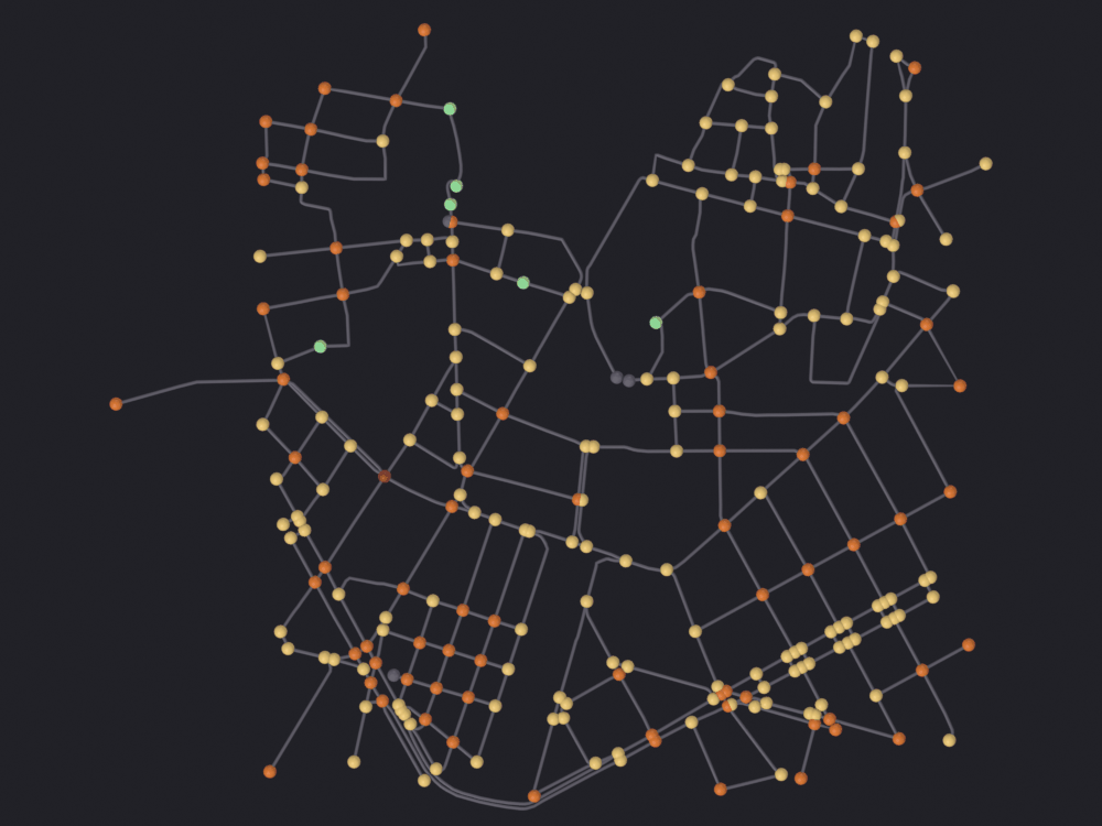
[PASS] 1_type_drive.png legible — 9.3% ink (healthy range 0.5–60%)
color range: (1.0, 5.0)nb.figure(networks['walk'], "renders/06_osmnx/2_type_walk",
look='ink', color_attribute="node_street_count")
print("color range:", sg.render.color_range(networks['walk'])) Skipping Split Edges: 'is_intersection' present, keeping streets continuous
Info: Geometry Nodes modifier added
Info: Attribute -> node_street_count · node_street_count -> turbo [log] [1 … 6] on Point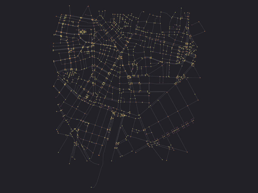
[PASS] 2_type_walk.png legible — 6.9% ink (healthy range 0.5–60%)
color range: (1.0, 6.0)
3 · Simplification
An OSM way is a polyline, and every vertex of it is a node in the raw graph. Most are not junctions, they are the shape of the street. simplify_graph removes them, merging each run of degree-2 nodes into a single edge whose geometry attribute keeps the shape. What comes out is the graph every street-network statistic in the literature is computed on: the raw one is a drawing of the road centerlines, the simplified one is the topology.
raw = download('POINT', 'drive', simplify=False)
raw.name = "Net_drive_raw"
G_raw = graph_cache.get_osmnx_graph(raw)
counts(G_raw, "raw (simplify=False)")

sg.graphs.activate(raw)
print("osmnx_simplify ->", bpy.ops.scigraphs.osmnx_simplify())
G_after = graph_cache.get_osmnx_graph(raw)
counts(G_after, "after osmnx_simplify")
counts(G_point, "simplify=True on download")

simplified = materialize(G_after, "Net_drive_simplified")

removed = G_raw.number_of_nodes() - G_after.number_of_nodes()
print()
print(f"nodes removed   {removed} of {G_raw.number_of_nodes()} "
      f"({100 * removed / G_raw.number_of_nodes():.1f} %)")
print(f"mesh vertices   {len(raw.data.vertices)} -> {len(simplified.data.vertices)}")
print(f"of which nodes  {raw.get('num_nodes')} -> {simplified.get('num_nodes')}")
print(f"mean edge span  {1000 * counts(G_raw)[2] / G_raw.number_of_edges():.1f} m"
      f"  ->  {1000 * counts(G_after)[2] / G_after.number_of_edges():.1f} m")

check("simplification removes most of the nodes",
      G_after.number_of_nodes() < G_raw.number_of_nodes() / 3)
check("it does not remove any street",
      abs(counts(G_after)[2] - counts(G_raw)[2]) < 0.02 * counts(G_raw)[2],
      "the length is carried into the merged edges' geometry")
Downloading OSM network (POINT)...
  Point: (39.46989822387695, -0.37630000710487366), radius: 600m
  Download completed in 0.24s
Total import time: 0.35s
  Nodes: 1,191, Edges: 1,330

Creating OSMnx graph: 1,191 nodes, 1,330 edges...
  Created 1,191 intersection vertices
    Created 1,000 edges...
  Created 1,283 street edges in 0.13s
Total OSMnx graph creation time: 0.14s
Graph saved to ~/.config/blender/5.2/scripts/addons/scigraphs_osmnx_cache/39.4699_-0.3763_drive.graphml
Graph cached to: ~/.config/blender/5.2/scripts/addons/scigraphs_osmnx_cache/39.4699_-0.3763_drive.graphml
Info: Downloading network from OpenStreetMap (POINT)...
Info: Graph cached as: 39.4699_-0.3763_drive.graphml
Info: Imported: 1191 intersections, 1330 street segments, 27.7 km total
  raw (simplify=False)             1191 nodes   1330 edges     27.7 km
Graph simplified: 1191 -> 254 nodes
Info: Simplified: 1191 -> 254 nodes
osmnx_simplify -> {'FINISHED'}
  after osmnx_simplify              254 nodes    358 edges     27.7 km
  simplify=True on download         243 nodes    375 edges     31.8 km

Creating OSMnx graph: 254 nodes, 358 edges...
  Created 254 intersection vertices
  Created 344 street edges in 0.01s
Total OSMnx graph creation time: 0.01s

nodes removed   937 of 1191 (78.7 %)
mesh vertices   1191 -> 1172
of which nodes  1191 -> 254
mean edge span  20.8 m  ->  77.3 m
[PASS] simplification removes most of the nodes
[PASS] it does not remove any street — the length is carried into the merged edges' geometryTrueTwo things that are not obvious
The operator does not touch the mesh. osmnx_simplify just reported a fall of about a thousand nodes, and the object it ran on still has every one of them as an intersection vertex: it replaced the graph in the in-memory cache (graph_operators.py:575-578) and stopped there. So does every operator in this family: osmnx_consolidate, osmnx_largest_component, osmnx_to_undirected, osmnx_to_digraph, osmnx_truncate_bbox, osmnx_truncate_polygon, osmnx_truncate_distance. That is what materialize() is for.
print(f"the graph in the cache   {G_after.number_of_nodes()} nodes")
print(f"the mesh it ran on       {raw.get('num_nodes')} intersection vertices, "
      f"{len(raw.data.vertices)} vertices in all")
check("the cleaning operators leave the mesh untouched",
      raw.get("num_nodes") == G_raw.number_of_nodes()
      != G_after.number_of_nodes(),
      "so a render taken now would draw the unsimplified network")
the graph in the cache 254 nodes
the mesh it ran on 1191 intersection vertices, 1191 vertices in all
[PASS] the cleaning operators leave the mesh untouched — so a render taken now would draw the unsimplified networkTrueSimplifying afterwards is not the same as simplifying on download, and the difference is not rounding. graph_from_point(simplify=True) simplifies inside the download pipeline, before the boundary truncation has finished; truncate_by_edge=True then keeps any edge with one endpoint inside the box, and a simplified edge spans a whole block rather than a few meters, so it reaches much further past the boundary and drags more network in behind it.
both = set(G_after.nodes) & set(G_point.nodes)
only_download = set(G_point.nodes) - set(G_after.nodes)
only_after = set(G_after.nodes) - set(G_point.nodes)


def median_radius(G, nodes):
    if not nodes:
        return float("nan")
    return float(np.median([
                 math.hypot((G.nodes[n]["y"] - CENTER[0]) * meters_per_degree,
                 (G.nodes[n]["x"] - CENTER[1]) * meters_per_degree
                 * math.cos(math.radians(CENTER[0])))
                 for n in nodes]))


print(f"in both                    {len(both):>5}   "
      f"median {median_radius(G_after, both):>5.0f} m from the center")
print(f"only simplify=True         {len(only_download):>5}   "
      f"median {median_radius(G_point, only_download):>5.0f} m")
print(f"only osmnx_simplify after  {len(only_after):>5}   "
      f"median {median_radius(G_after, only_after):>5.0f} m")
print(f"the request was for {RADIUS_M} m")
print(f"total length {counts(G_point)[2]:.1f} km on download vs "
      f"{counts(G_after)[2]:.1f} km simplifying afterwards")

check("the two simplifications disagree at the boundary",
      bool(only_download or only_after)
      and median_radius(G_point, only_download) > 0.9 * RADIUS_M,
      "the nodes they disagree about sit at the edge of the download")
in both 203 median 573 m from the center
only simplify=True 40 median 752 m
only osmnx_simplify after 51 median 704 m
the request was for 600 m
total length 31.8 km on download vs 27.7 km simplifying afterwards
[PASS] the two simplifications disagree at the boundary — the nodes they disagree about sit at the edge of the downloadTrueBefore and after
The shape does not change, the geometry is preserved; the nodes do. The raw figure has a bead on every bend, the simplified one only where streets meet. The color is node_degree: in the raw graph almost every node has degree 2, and afterwards almost none does.
for obj, G, label in ((raw, G_raw, "raw"), (simplified, G_after, "simplified")):
    degrees = dict(nx.Graph(G).degree())
    node_attribute(obj, degrees, "node_degree")
    values = np.array(list(degrees.values()))
    print(f"  {label:<11} mean degree {values.mean():.2f}, "
          f"{100 * (values == 2).mean():>4.1f} % of nodes have degree 2, "
          f"max {values.max()}")
raw mean degree 2.15, 79.3 % of nodes have degree 2, max 5
simplified mean degree 2.71, 3.9 % of nodes have degree 2, max 5nb.figure(raw, "renders/06_osmnx/3_simplify_before",
look='ink', color_attribute="node_degree") Skipping Split Edges: 'is_intersection' present, keeping streets continuous
Info: Geometry Nodes modifier added
Info: Attribute -> node_degree · node_degree -> turbo [log] [1 … 5] on Point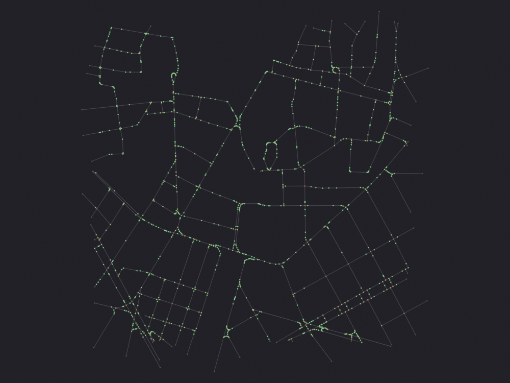
[PASS] 3_simplify_before.png legible — 3.6% ink (healthy range 0.5–60%)nb.figure(simplified, "renders/06_osmnx/4_simplify_after",
look='ink', color_attribute="node_degree") Skipping Split Edges: 'is_intersection' present, keeping streets continuous
Info: Geometry Nodes modifier added
Info: Attribute -> node_degree · node_degree -> turbo [log] [1 … 5] on Point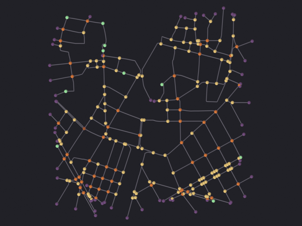
[PASS] 4_simplify_after.png legible — 8.5% ink (healthy range 0.5–60%)4 · Consolidation, and what a tolerance costs
Simplification removes nodes that are not junctions; consolidation goes after the opposite problem, one junction mapped as several nodes. A dual carriageway crossing another is four nodes in OSM and one intersection on the ground; a roundabout is a ring of nodes and one intersection. osmnx_consolidate buffers every node by a tolerance in meters, merges what overlaps, and rebuilds the edges between the survivors.
It enforces two preconditions: the graph must be projected, because a tolerance in meters is meaningless in degrees (graph_operators.py:621-626), and it must be directed (graph_operators.py:628-630), so this has to happen before any to_undirected.
And one that nothing enforces: once projected the graph is in UTM meters, and materialize(), like every other route into a Blender mesh, reads x/y as longitude and latitude. A projected graph silently draws as a mesh tens of thousands of Blender units across, so a consolidated graph has to go back to EPSG:4326 before it can be looked at.
sg.graphs.activate(simplified)
print("osmnx_project_graph ->",
      bpy.ops.scigraphs.osmnx_project_graph(crs_preset='AUTO_UTM'))
G_projected = graph_cache.get_osmnx_graph(simplified)
print(f"  crs {simplified.get('osmnx_crs')},  "
      f"projected {simplified.get('osmnx_projected')}")
sample = next(iter(G_projected.nodes(data=True)))[1]
print(f"  a node is now at x={sample['x']:,.1f} y={sample['y']:,.1f} "
      "(meters, not degrees)")
Graph projected to EPSG:32630
Info: Graph projected to EPSG:32630
osmnx_project_graph -> {'FINISHED'}
crs EPSG:32630, projected True
a node is now at x=725,813.2 y=4,371,905.8 (meters, not degrees)TOLERANCES = (5, 10, 20, 40)
consolidated = {}
print(f" {'tolerance':>9} {'nodes':>6} {'edges':>6} {'kept':>6} "
f"{'moved p50':>10} {'moved max':>10}")
for tolerance in TOLERANCES:
graph_cache.store_osmnx_graph(simplified, G_projected.copy())
result = bpy.ops.scigraphs.osmnx_consolidate(tolerance=float(tolerance))
if 'FINISHED' not in result:
print(f" {tolerance:>9} {result}")
continue
G_c = graph_cache.get_osmnx_graph(simplified)
shifts, merged = [], {}
for node, data in G_c.nodes(data=True):
originals = data.get("osmid_original", data.get("osmid", node))
if isinstance(originals, str):
originals = [int(t) for t in originals.strip("[]").split(",")
if t.strip().lstrip("-").isdigit()]
elif not isinstance(originals, (list, tuple, set)):
originals = [originals]
merged[node] = len(originals)
for original in originals:
if original in G_projected.nodes:
shifts.append(math.hypot(
data["x"] - G_projected.nodes[original]["x"],
data["y"] - G_projected.nodes[original]["y"]))
shifts = np.array(shifts) if shifts else np.zeros(1)
consolidated[tolerance] = (G_c, merged, shifts)
print(f" {tolerance:>9} {G_c.number_of_nodes():>6} "
f"{G_c.number_of_edges():>6} "
f"{100 * G_c.number_of_nodes() / G_projected.number_of_nodes():>5.0f}% "
f"{np.median(shifts):>9.1f} m {shifts.max():>9.1f} m")
graph_cache.store_osmnx_graph(simplified, G_projected)
check("every tolerance consolidated something",
len(consolidated) == len(TOLERANCES))
check("a node can move further than the tolerance",
any(shift.max() > tolerance
for tolerance, (_G, _m, shift) in consolidated.items()),
"a chain of nodes within the tolerance collapses to one point that "
"need not be within the tolerance of any of them") tolerance nodes edges kept moved p50 moved max
Intersections consolidated: 254 -> 239 nodes
Info: Consolidated: 254 -> 239 nodes
5 239 342 94% 0.0 m 5.0 m
Intersections consolidated: 254 -> 205 nodes
Info: Consolidated: 254 -> 205 nodes
10 205 307 81% 0.0 m 18.8 m
Intersections consolidated: 254 -> 160 nodes
Info: Consolidated: 254 -> 160 nodes
20 160 245 63% 3.0 m 70.5 m
Intersections consolidated: 254 -> 67 nodes
Info: Consolidated: 254 -> 67 nodes
40 67 113 26% 65.2 m 302.5 m
[PASS] every tolerance consolidated something
[PASS] a node can move further than the tolerance — a chain of nodes within the tolerance collapses to one point that need not be within the tolerance of any of themTrueRead the last two columns, not the first. The distance a node moves is the price of the falling node count, and it is not bounded by the tolerance you set: t merges nodes within t of each other, so a chain of them (a roundabout, a long staggered junction, a slip road) collapses to a single point that can sit much further than t from any of the originals. At a large enough tolerance a whole short street becomes a node, and the edge that was that street goes with it.
There is no universally correct value:
- 10 m is OSMnx’s default and about right for an ordinary urban grid;
- a medieval center wants less; the blocks here are short, and 20 m is already merging junctions that a pedestrian would tell apart;
- a motorway interchange wants 30 to 50 m, or the slip roads stay as separate intersections and every centrality measure is diluted across them;
- quote whatever you choose next to the number, because a node count without a tolerance is not reproducible.
Consolidation also throws away node identity: the survivor gets a new integer id and keeps the originals in osmid_original, so anything joined to the graph by OSM node id has to be re-joined. Notebook 09 hits this when it attaches points of interest.
The figure, colored by how many nodes each one swallowed
node_merged is 1 where consolidation changed nothing and higher where it collapsed a cluster. The merges concentrate at a handful of large junctions while most of the network is untouched, so the long tail is clipped at the top percentile rather than allowed to flatten everything else into the bottom stop of the ramp.
CHOSEN_TOLERANCE = 20
G_c, merged, shifts = consolidated[CHOSEN_TOLERANCE]

G_c_wgs = ox.projection.project_graph(G_c, to_crs="epsg:4326")
consolidated_obj = materialize(G_c_wgs, f"Net_consolidated_{CHOSEN_TOLERANCE}m")
written, array = node_attribute(consolidated_obj, merged, "node_merged")

multiple = sum(1 for v in merged.values() if v > 1)
print(f"nodes that swallowed more than one  {multiple} of {len(merged)} "
      f"({100 * multiple / len(merged):.0f} %)")
print(f"largest single merge                {max(merged.values())} nodes into one")
print(f"attribute written on                {written} intersections")
print(f"edges lost to the merge             "
      f"{G_projected.number_of_edges() - G_c.number_of_edges()}")

check("the consolidated graph is back in degrees",
      abs(float(next(iter(G_c_wgs.nodes(data=True)))[1]["x"])) < 180.0,
      "or the mesh would be tens of thousands of Blender units across")
Creating OSMnx graph: 160 nodes, 245 edges...
  Created 160 intersection vertices
  Created 223 street edges in 0.01s
Total OSMnx graph creation time: 0.01s
nodes that swallowed more than one  37 of 160 (23 %)
largest single merge                11 nodes into one
attribute written on                160 intersections
edges lost to the merge             113
[PASS] the consolidated graph is back in degrees — or the mesh would be tens of thousands of Blender units acrossTruenb.figure(consolidated_obj, "renders/06_osmnx/5_consolidated",
look='ink', color_attribute="node_merged",
clip_high_pct=98) Skipping Split Edges: 'is_intersection' present, keeping streets continuous
Info: Geometry Nodes modifier added
Info: Attribute -> node_merged · node_merged -> turbo [log] [1 … 7] on Point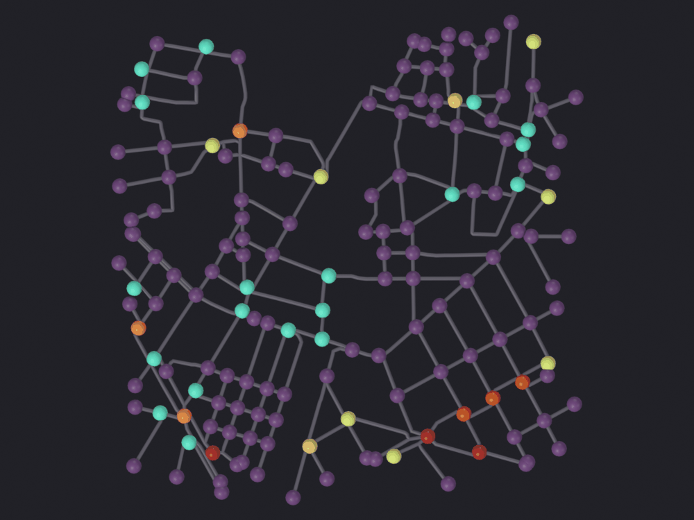
[PASS] 5_consolidated.png legible — 14.7% ink (healthy range 0.5–60%)5 · Direction, and the pieces that are not connected
An OSMnx street graph is a MultiDiGraph: a one-way street is one directed edge, a two-way street is two, and a pair of parallel edges between the same nodes is how a divided street or a service loop is spelled. Three operators change that shape, each right for a different question.
walkable = download('POINT', 'walk', retain_all=True)
walkable.name = "Net_walk_all_components"
G_walk = graph_cache.get_osmnx_graph(walkable)
counts(G_walk, "walk, retain_all=True")

sg.graphs.activate(walkable)
print("osmnx_to_undirected ->", bpy.ops.scigraphs.osmnx_to_undirected())
G_undirected = graph_cache.get_osmnx_graph(walkable)
print(f"  {type(G_undirected).__name__:<14} "
      f"{G_undirected.number_of_edges():>5} edges "
      f"({100 * G_undirected.number_of_edges() / G_walk.number_of_edges():.0f} % "
      "of the directed count)")

graph_cache.store_osmnx_graph(walkable, G_walk)
print("osmnx_to_digraph ->", bpy.ops.scigraphs.osmnx_to_digraph())
G_digraph = graph_cache.get_osmnx_graph(walkable)
print(f"  {type(G_digraph).__name__:<14} "
      f"{G_digraph.number_of_edges():>5} edges "
      f"({G_walk.number_of_edges() - G_digraph.number_of_edges()} parallel "
      "edges collapsed, and not recoverable)")
graph_cache.store_osmnx_graph(walkable, G_walk)

check("to_undirected halves a fully bidirectional network",
      G_undirected.number_of_edges() <= G_walk.number_of_edges() / 2 + 1)
check("to_digraph drops the parallel edges",
      G_digraph.number_of_edges() < G_walk.number_of_edges())
Downloading OSM network (POINT)...
  retain_all: True (disconnected components kept)
  Point: (39.46989822387695, -0.37630000710487366), radius: 600m
  Download completed in 1.34s
Total import time: 1.62s
  Nodes: 1,600, Edges: 4,732

Creating OSMnx graph: 1,600 nodes, 4,732 edges...
  Created 1,600 intersection vertices
    Created 1,000 edges...
    Created 2,000 edges...
  Created 2,346 street edges in 0.33s
Total OSMnx graph creation time: 0.34s
Graph saved to ~/.config/blender/5.2/scripts/addons/scigraphs_osmnx_cache/39.4699_-0.3763_walk.graphml
Graph cached to: ~/.config/blender/5.2/scripts/addons/scigraphs_osmnx_cache/39.4699_-0.3763_walk.graphml
Info: Downloading network from OpenStreetMap (POINT)...
Info: Graph cached as: 39.4699_-0.3763_walk.graphml
Info: Imported: 1600 intersections, 4732 street segments, 148.9 km total
  walk, retain_all=True            1600 nodes   4732 edges    148.9 km
Converted to undirected graph
Info: Converted to undirected graph
osmnx_to_undirected -> {'FINISHED'}
  MultiGraph      2366 edges (50 % of the directed count)
Converted to DiGraph (weight: length)
Info: Converted to DiGraph (by length)
osmnx_to_digraph -> {'FINISHED'}
  DiGraph         4690 edges (42 parallel edges collapsed, and not recoverable)
[PASS] to_undirected halves a fully bidirectional network
[PASS] to_digraph drops the parallel edgesTrueosmnx_to_undirectedcollapses each reciprocal pair into one edge. Use it for anything about the street rather than travel along it: total length, circuity, orientation, street counts. OSMnx converts internally before several of its own statistics, andosmnx_circuitydoes the same.osmnx_to_digraphkeeps direction but throws away multiplicity, choosing the shortest of each parallel bundle. It exists because many NetworkX algorithms refuse a multigraph, and it loses edges silently: on a network with many divided streets that loss is not small.- Neither is reversible.
convert.ensure_multidigraphrebuilds aMultiDiGraphshape afterwards so OSMnx’s own helpers keep working, but the edgesto_digraphdropped do not come back.
osmnx_to_undirectedsetsobj["is_directed"] = False, which the direction arrows and the directed-analysis panels read, and does not rebuild the mesh: the arrows vanish from a network whose drawn geometry has not changed.
Components, and what retain_all is for
retain_all=False, the default and what every other download here used, tells OSMnx to keep only the largest weakly connected component. That is usually right, and it is always a decision. The download above set retain_all=True, so this graph still has everything.
weak = sorted(nx.weakly_connected_components(G_walk), key=len, reverse=True)
strong = sorted(nx.strongly_connected_components(G_walk), key=len, reverse=True)

print(f"nodes                {G_walk.number_of_nodes()}")
print(f"weakly connected     {len(weak)} components, "
      f"sizes {[len(c) for c in weak[:8]]}{' …' if len(weak) > 8 else ''}")
print(f"strongly connected   {len(strong)} components, "
      f"sizes {[len(c) for c in strong[:8]]}{' …' if len(strong) > 8 else ''}")
print(f"the largest weak component holds "
      f"{100 * len(weak[0]) / G_walk.number_of_nodes():.1f} % of the nodes")

sg.graphs.activate(walkable)
print("\nosmnx_largest_component(strongly=False) ->",
      bpy.ops.scigraphs.osmnx_largest_component(strongly=False))
G_weak = graph_cache.get_osmnx_graph(walkable)
counts(G_weak, "largest weak component")

graph_cache.store_osmnx_graph(walkable, G_walk)
print("osmnx_largest_component(strongly=True) ->",
      bpy.ops.scigraphs.osmnx_largest_component(strongly=True))
G_strong = graph_cache.get_osmnx_graph(walkable)
counts(G_strong, "largest strong component")
graph_cache.store_osmnx_graph(walkable, G_walk)
nodes 1600
weakly connected 10 components, sizes [1582, 2, 2, 2, 2, 2, 2, 2] …
strongly connected 10 components, sizes [1582, 2, 2, 2, 2, 2, 2, 2] …
the largest weak component holds 98.9 % of the nodes
Extracted largest component: 1600 -> 1582 nodes
Info: Largest component: 1582 / 1600 nodes
osmnx_largest_component(strongly=False) -> {'FINISHED'}
largest weak component 1582 nodes 4714 edges 147.6 km
Extracted largest component: 1600 -> 1582 nodes
Info: Largest component: 1582 / 1600 nodes
osmnx_largest_component(strongly=True) -> {'FINISHED'}
largest strong component 1582 nodes 4714 edges 147.6 kmWhen is the largest-component filter the right call?
- Almost always, for routing: a disconnected fragment is somewhere the router cannot reach, and
nx.shortest_pathraises. Notebook 08 depends on this having been done. - Almost always, for centrality: betweenness on a disconnected graph is computed per component and is not comparable across them.
- Not, when the fragments are the subject: islands, a pedestrianized precinct reachable only on foot, a network deliberately cut by a barrier.
- Not, when the fragments are an artifact of the boundary. Almost all the small components here are stubs of exactly two nodes, a street that leaves the download box and comes back in: disconnected in this extract, not in the world. Download wider and truncate, as section 8 does.
kept = len(weak[0])
print(f"largest component     {kept} nodes")
print(f"discarded             {G_walk.number_of_nodes() - kept} nodes in "
      f"{len(weak) - 1} fragments, sizes "
      f"{sorted({len(c) for c in weak[1:]})}")
print(f"discarded street      {counts(G_walk)[2] - counts(G_weak)[2]:.2f} km "
      f"of {counts(G_walk)[2]:.1f} km "
      f"({100 * (counts(G_walk)[2] - counts(G_weak)[2]) / counts(G_walk)[2]:.1f} %)")

check("the largest component keeps almost everything here",
      kept / G_walk.number_of_nodes() > 0.95,
      f"{100 * kept / G_walk.number_of_nodes():.1f} % of the nodes")
largest component 1582 nodes
discarded 18 nodes in 9 fragments, sizes [2]
discarded street 1.27 km of 148.9 km (0.9 %)
[PASS] the largest component keeps almost everything here — 98.9 % of the nodesTrueWeak and strong, on a network where they differ
Weak connectivity ignores direction: two nodes are together if you could get between them disregarding the one-way signs. Strong connectivity respects them, so the difference is the set of places you can drive into but not out of, or out of but not into.
On the pedestrian network above the two coincide, because every footway is two-way, which is a useful check that the walk filter did what it claims and is why that graph could not show this.
G_drive = graph_cache.get_osmnx_graph(networks['drive'])
drive_weak = sorted(nx.weakly_connected_components(G_drive), key=len,
                    reverse=True)
drive_strong = sorted(nx.strongly_connected_components(G_drive), key=len,
                      reverse=True)

print(f"drive network        {G_drive.number_of_nodes()} nodes")
print(f"weakly connected     {len(drive_weak)} component(s), "
      f"sizes {[len(c) for c in drive_weak[:4]]}")
print(f"strongly connected   {len(drive_strong)} components, "
      f"largest {len(drive_strong[0])}, and "
      f"{sum(1 for c in drive_strong if len(c) == 1)} single nodes")
print(f"so {100 * (1 - len(drive_strong[0]) / G_drive.number_of_nodes()):.0f} % "
      "of the intersections are not mutually reachable with the rest")

check("the drive network is weakly but not strongly connected",
      len(drive_weak) == 1 and len(drive_strong) > 1,
      f"one weak component, {len(drive_strong)} strong ones")
drive network 243 nodes
weakly connected 1 component(s), sizes [243]
strongly connected 46 components, largest 198, and 45 single nodes
so 19 % of the intersections are not mutually reachable with the rest
[PASS] the drive network is weakly but not strongly connected — one weak component, 46 strong onesTrueThose single-node strong components are the far end of a one-way street, a service entrance, an intersection whose only exit was truncated at the boundary. Nothing reports them, and section 8 shows one of them silently emptying a catchment.
node_balance is out-degree minus in-degree: zero where as many ways lead out as in, negative where a node absorbs more than it emits, positive where it emits more. On turbo that runs blue through green to red, and the pattern it draws is the one-way system: pairs of opposite-signed nodes strung along the streets that only run one way, green where traffic can turn around.
balance = {n: G_drive.out_degree(n) - G_drive.in_degree(n) for n in G_drive}
node_attribute(networks['drive'], balance, "node_balance")

values = np.array(list(balance.values()))
print(f"out-degree minus in-degree: {values.min()} to {values.max()}")
for value in range(int(values.min()), int(values.max()) + 1):
    share = 100 * (values == value).mean()
    print(f"  {value:>+3}  {(values == value).sum():>4} nodes  {share:>5.1f} %")
no_exit = [n for n in G_drive if G_drive.out_degree(n) == 0]
no_entry = [n for n in G_drive if G_drive.in_degree(n) == 0]
print(f"of which no way out at all  {len(no_exit)} nodes")
print(f"          no way in at all  {len(no_entry)} nodes")

check("the balance is not everywhere zero",
      float((values != 0).mean()) > 0.5,
      f"{100 * (values != 0).mean():.0f} % of intersections are asymmetric")
out-degree minus in-degree: -2 to 2
-2 11 nodes 4.5 %
-1 77 nodes 31.7 %
+0 66 nodes 27.2 %
+1 79 nodes 32.5 %
+2 10 nodes 4.1 %
of which no way out at all 17 nodes
no way in at all 15 nodes
[PASS] the balance is not everywhere zero — 73 % of intersections are asymmetricTruenb.figure(networks['drive'], "renders/06_osmnx/6_direction",
look='ink', color_attribute="node_balance") Skipping Split Edges: 'is_intersection' present, keeping streets continuous
Info: Geometry Nodes modifier added
Info: Attribute -> node_balance · node_balance -> turbo [log] [-2 … 2] on Point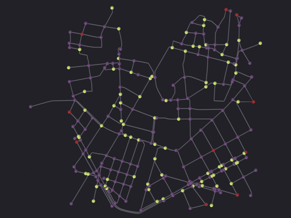
[PASS] 6_direction.png legible — 9.2% ink (healthy range 0.5–60%)6 · The basic statistics, and what they mean here
osmnx_basic_stats wraps ox.basic_stats and writes each result onto the object as osmnx_stat_*. The densities among them need an area, which the operator takes from osmnx_network_area when it is set and otherwise estimates as the convex hull of the nodes, through osmnx_estimate_area.
The hull is not the study area. With truncate_by_edge=True the network reaches past the 600 m disc, so the hull is larger and every density comes out correspondingly smaller. If the study area is a district boundary or a census tract, set osmnx_network_area by hand first.
stats_obj = materialize(G_point, "Net_drive_stats")
sg.graphs.activate(stats_obj)

props.osmnx_network_area = 0.0
print("osmnx_estimate_area ->", bpy.ops.scigraphs.osmnx_estimate_area())
print(f"  convex hull {props.osmnx_network_area:.3f} km2, against "
      f"{math.pi * (RADIUS_M / 1000) ** 2:.3f} km2 for the requested disc "
      f"({100 * props.osmnx_network_area / (math.pi * (RADIUS_M / 1000) ** 2) - 100:+.0f} %)")

print("osmnx_basic_stats ->", bpy.ops.scigraphs.osmnx_basic_stats())
for key in sorted(k for k in stats_obj.keys() if k.startswith("osmnx_stat_")):
    print(f"  {key[len('osmnx_stat_'):]:<30} {stats_obj[key]}")

check("the statistics landed on the object",
      bool(stats_obj.get("osmnx_stats_calculated")))
Creating OSMnx graph: 243 nodes, 375 edges...
  Created 243 intersection vertices
  Created 361 street edges in 0.01s
Total OSMnx graph creation time: 0.01s
Estimated network area: 2.02 km2
Info: Estimated network area: 2.02 km2
osmnx_estimate_area -> {'FINISHED'}
  convex hull 2.021 km2, against 1.131 km2 for the requested disc (+79 %)
Basic stats calculated: 243 nodes, 375 edges
Info: Nodes: 243, Edges: 375, Length: 31.8 km
osmnx_basic_stats -> {'FINISHED'}
  avg_degree                     3.09
  avg_edge_length_m              84.8
  circuity_avg                   1.041
  dead_end_count                 0
  edge_density_per_km2           15722.38
  intersection_count             239
  n_edges                        375
  n_nodes                        243
  node_density_per_km2           120.21
  street_density_km_per_km2      15339.75
  street_segments_per_node       3.26
  total_length_km                31.78
[PASS] the statistics landed on the objectTrueWhat the interesting ones mean for a street network:
street_segments_per_node: the mean number of physical streets at a junction, computed on the undirected graph, so it describes the layout and not the one-way system. Around 3 is normal urban, mostly T-junctions with some crossroads; below 2.5 is cul-de-sac suburbia; above 3.5 a dense grid.intersection_countanddead_end_countsplit the nodes into junctions and stubs, and are meaningful only on a simplified graph: on a raw one nearly every node is a degree-2 non-junction.circuity_avg: the mean ratio of edge length to the straight-line distance between its endpoints. 1.0 is perfectly straight segments; a few percent above is a mostly-rectilinear old town. It is a shape statistic and not a detour factor: a perfect grid has circuity 1.0 and still makes you walk 1.4 times the crow-flies distance.avg_edge_length_m: the block size, and the number most sensitive to everything above. Simplification multiplies it several times over, consolidation raises it again.
Two of the density labels are wrong, by a factor of a thousand.
ox.basic_statsreturnsedge_density_kmandstreet_density_kmin meters of network per square kilometer.SciGraphs/core/osmnx/stats.py(lines 38-40) copies them intoedge_density_per_km2andstreet_density_km_per_km2, whose names promise a count of edges per km² and kilometers per km². Divide by 1000 for the figure street-network papers quote.node_density_per_km2is what its name says.
The two are measured on different graphs: edge_density counts the directed edges, street_density the undirected streets. Their ratio measures how one-way a network is: 2.0 for a fully two-way street system, barely above 1 for a medieval center where almost everything runs one way.
area_km2 = float(props.osmnx_network_area)
edge_density = float(stats_obj.get("osmnx_stat_edge_density_per_km2", 0.0))
street_density = float(stats_obj.get("osmnx_stat_street_density_km_per_km2", 0.0))
total_km = float(stats_obj.get("osmnx_stat_total_length_km", 0.0))

print(f"edge_density_per_km2, as reported    {edge_density:>12,.0f}")
print(f"total edge length / area             "
      f"{1000 * total_km / area_km2:>12,.0f}   m per km2")
print(f"street_density_km_per_km2            {street_density:>12,.0f}")
print(f"the figure a paper would quote       "
      f"{street_density / 1000:>12,.1f}   km of street per km2")
print(f"directed / undirected length         "
      f"{edge_density / street_density:>12,.2f}   "
      f"(2.0 would be an entirely two-way network)")

check("the density labeled km/km2 is really m/km2",
      abs(edge_density - 1000 * total_km / area_km2)
      < 0.01 * edge_density,
      "a thousand times the number the name promises")
edge_density_per_km2, as reported 15,722
total edge length / area 15,721 m per km2
street_density_km_per_km2 15,340
the figure a paper would quote 15.3 km of street per km2
directed / undirected length 1.02 (2.0 would be an entirely two-way network)
[PASS] the density labeled km/km2 is really m/km2 — a thousand times the number the name promisesTrue7 · The round trip, and whether it is lossless
graph_to_gdfs turns the graph into two GeoDataFrames, nodes indexed by osmid and edges by (u, v, key), and gdfs_to_graph turns them back. That pair is the seam between OSMnx and every other geospatial tool. Three versions of the same trip below, and they do not all pass.
gdf_nodes, gdf_edges = convert.graph_to_gdfs(G_point)

print(f"nodes {len(gdf_nodes):>5}  index {gdf_nodes.index.names}")
print(f"      {list(gdf_nodes.columns)}")
print(f"edges {len(gdf_edges):>5}  index {gdf_edges.index.names}")
print(f"      {list(gdf_edges.columns)}")
nodes 243 index ['osmid']
['y', 'x', 'street_count', 'highway', 'geometry']
edges 375 index ['u', 'v', 'key']
['osmid', 'highway', 'lanes', 'maxspeed', 'name', 'oneway', 'reversed', 'length', 'geometry', 'width', 'tunnel', 'access', 'junction']In memory
The strict test: same node set, same (u, v, key) triples, and the same attribute names on both sides.
G_back = convert.graph_from_gdfs(gdf_nodes, gdf_edges)


def edge_attrs(G):
    keys = set()
    for *_ids, data in G.edges(keys=True, data=True):
        keys |= set(data)
    return keys


def node_attrs(G):
    keys = set()
    for _n, data in G.nodes(data=True):
        keys |= set(data)
    return keys


print(f"nodes           {G_point.number_of_nodes()} -> {G_back.number_of_nodes()}")
print(f"edges           {G_point.number_of_edges()} -> {G_back.number_of_edges()}")
print(f"node ids equal  {set(G_point.nodes) == set(G_back.nodes)}")
print(f"edge keys equal "
      f"{set(G_point.edges(keys=True)) == set(G_back.edges(keys=True))}")
print(f"node attributes {sorted(node_attrs(G_point))}")
print(f"          after {sorted(node_attrs(G_back))}")
print(f"edge attributes {sorted(edge_attrs(G_point))}")
print(f"          after {sorted(edge_attrs(G_back))}")

lost = set(G_point.graph) - set(G_back.graph)
print(f"\ngraph-level metadata before {sorted(G_point.graph)}")
print(f"                      after {sorted(G_back.graph)}")
print(f"                       lost {sorted(lost)}")

check("the node and edge sets survive the round trip",
      set(G_point.nodes) == set(G_back.nodes)
      and set(G_point.edges(keys=True)) == set(G_back.edges(keys=True)))
check("every node and edge attribute survives",
      node_attrs(G_point) == node_attrs(G_back)
      and edge_attrs(G_point) == edge_attrs(G_back))
check("the graph-level metadata does not", bool(lost),
      f"{sorted(lost)} are dropped; `graph_from_gdfs` keeps only the CRS "
      "unless `graph_attrs=` is passed")
nodes 243 -> 243
edges 375 -> 375
node ids equal True
edge keys equal True
node attributes ['highway', 'street_count', 'x', 'y']
after ['highway', 'street_count', 'x', 'y']
edge attributes ['access', 'geometry', 'highway', 'junction', 'lanes', 'length', 'maxspeed', 'name', 'oneway', 'osmid', 'reversed', 'tunnel', 'width']
after ['access', 'geometry', 'highway', 'junction', 'lanes', 'length', 'maxspeed', 'name', 'oneway', 'osmid', 'reversed', 'tunnel', 'width']
graph-level metadata before ['created_date', 'created_with', 'crs', 'simplified']
after ['crs']
lost ['created_date', 'created_with', 'simplified']
[PASS] the node and edge sets survive the round trip
[PASS] every node and edge attribute survives
[PASS] the graph-level metadata does not — ['created_date', 'created_with', 'simplified'] are dropped; `graph_from_gdfs` keeps only the CRS unless `graph_attrs=` is passedTrueNode and edge identity, geometry and every per-feature attribute come back exactly. What is dropped is G.graph, and the entry that matters there is simplified, the flag osmnx_simplify checks before refusing to run twice (graph_operators.py:555). A graph that has been through the GeoDataFrame round trip can be simplified again; OSMnx will oblige, and the result is wrong in ways that are hard to see. created_date and created_with go with it, which is provenance rather than data, and provenance has its own notebook (07).
Through files, via the operators
osmnx_graph_to_gdfs writes two GeoJSONs and osmnx_gdfs_to_graph reads two: the file version of the pair above, and the obvious way to get a network out to QGIS and back. They do not compose.
out_dir = nb.out("10_osmnx")
out_dir.mkdir(parents=True, exist_ok=True)
base = out_dir / "roundtrip"

sg.graphs.activate(networks['drive'])
print("osmnx_graph_to_gdfs ->",
      bpy.ops.scigraphs.osmnx_graph_to_gdfs(filepath=str(base) + ".geojson"))
for path in sorted(out_dir.glob("roundtrip_*.geojson")):
    print(f"  {path.name:<26} {path.stat().st_size / 1e3:>8.1f} kB")

file_nodes = gpd.read_file(base.with_name("roundtrip_nodes.geojson"))
file_edges = gpd.read_file(base.with_name("roundtrip_edges.geojson"))
print(f"\nread back: nodes index {file_nodes.index.names}, "
      f"columns {list(file_nodes.columns)[:5]} …")
print(f"           edges index {file_edges.index.names}, "
      f"columns {list(file_edges.columns)[:5]} …")

failure = None
try:
    convert.graph_from_gdfs(file_nodes, file_edges)
except Exception as exc:                    # noqa: BLE001 - this is the point
    failure = f"{type(exc).__name__}: {exc}"
print(f"\ngraph_from_gdfs on what was just written -> {failure or 'OK'}")

check("the operator pair cannot read its own output", failure is not None,
      "GeoJSON has no MultiIndex, so u, v, key and osmid come back as "
      "plain columns and graph_from_gdfs rejects them")
Info: GeoDataFrames saved: 243 nodes, 375 edges
osmnx_graph_to_gdfs -> {'FINISHED'}
roundtrip_edges.geojson 200.8 kB
roundtrip_nodes.geojson 50.3 kB
read back: nodes index [None], columns ['osmid', 'y', 'x', 'street_count', 'highway'] …
edges index [None], columns ['u', 'v', 'key', 'osmid', 'highway'] …
graph_from_gdfs on what was just written -> IndexError: Too many levels: Index has only 1 level, not 2
[PASS] the operator pair cannot read its own output — GeoJSON has no MultiIndex, so u, v, key and osmid come back as plain columns and graph_from_gdfs rejects themTrueDefect.
SCIGRAPHS_OT_GraphToGDFscallsto_file(..., driver='GeoJSON')(graph_operators.py:1065-1066), and GeoJSON has no concept of an index, so the MultiIndex is flattened into ordinary columns.SCIGRAPHS_OT_GDFsToGraphthen callsgpd.read_fileand hands the result straight tograph_from_gdfs(graph_operators.py:1108-1111), which requiresosmidas the node index and(u, v, key)as a three-level edge MultiIndex. The result isIndexError: Too many levels.
Restoring the index is one line each way, and it is the first of three layers. The second: GDAL types a column by the widest thing in it, and a simplified graph has a handful of edges whose highway or name is a list of the ways that were merged, so the whole column is written as a string list. The arrays that reading produces are not lists either, and graph_from_gdfs rejects them.
indexed_nodes = file_nodes.set_index("osmid")
indexed_edges = file_edges.set_index(["u", "v", "key"])

second = None
try:
    convert.graph_from_gdfs(indexed_nodes, indexed_edges)
except Exception as exc:                    # noqa: BLE001 - also the point
    second = f"{type(exc).__name__}: {exc}"
print(f"with the index restored -> {second or 'OK'}")


def delist(gdf):
    """Turn the arrays GeoJSON reading produces back into plain lists."""
    frame = gdf.copy()
    for column in frame.columns:
        if column == frame.geometry.name:
            continue
        if frame[column].map(lambda v: isinstance(v, np.ndarray)).any():
            frame[column] = frame[column].map(
                lambda v: list(v) if isinstance(v, np.ndarray) else v)
    return frame


G_from_file = convert.graph_from_gdfs(delist(indexed_nodes),
                                      delist(indexed_edges))
print(f"and with the arrays unpacked -> {G_from_file.number_of_nodes()} nodes, "
      f"{G_from_file.number_of_edges()} edges")
print(f"node ids equal  {set(G_from_file.nodes) == set(G_point.nodes)}")
print(f"edge keys equal "
      f"{set(G_from_file.edges(keys=True)) == set(G_point.edges(keys=True))}")

check("the topology survives the file round trip once both are fixed",
      set(G_from_file.nodes) == set(G_point.nodes)
      and set(G_from_file.edges(keys=True))
      == set(G_point.edges(keys=True)))
with the index restored -> ValueError: The truth value of an array with more than one element is ambiguous. Use a.any() or a.all()
and with the arrays unpacked -> 243 nodes, 375 edges
node ids equal True
edge keys equal True
[PASS] the topology survives the file round trip once both are fixedTrueThe third layer is the one no amount of re-indexing gets back: the values themselves changed type. An edge whose highway was the string "secondary" now has the list ["secondary"], because one edge elsewhere in the column needed a list and GeoJSON cannot say that only some rows are lists. Anything comparing data["highway"] == "secondary", which is most code that touches OSM tags, silently stops matching.
def kinds(graph, attribute):
    counts_ = {"scalar": 0, "list": 0, "missing": 0}
    for *_ids, data in graph.edges(keys=True, data=True):
        value = data.get(attribute)
        if value is None:
            counts_["missing"] += 1
        elif isinstance(value, (list, tuple, np.ndarray)):
            counts_["list"] += 1
        else:
            counts_["scalar"] += 1
    return counts_


for attribute in ("highway", "name", "osmid"):
    before, after = kinds(G_point, attribute), kinds(G_from_file, attribute)
    print(f"  {attribute:<8} before {before}")
    print(f"  {'':<8} after  {after}")

check("scalar tags come back as one-element lists",
      kinds(G_from_file, "highway")["scalar"]
      < kinds(G_point, "highway")["scalar"],
      "GeoJSON promotes the whole column to a list type")
highway before {'scalar': 372, 'list': 3, 'missing': 0}
after {'scalar': 0, 'list': 375, 'missing': 0}
name before {'scalar': 337, 'list': 35, 'missing': 3}
after {'scalar': 0, 'list': 372, 'missing': 3}
osmid before {'scalar': 290, 'list': 85, 'missing': 0}
after {'scalar': 290, 'list': 85, 'missing': 0}
[PASS] scalar tags come back as one-element lists — GeoJSON promotes the whole column to a list typeTrueSo the GeoJSON pair is for looking at the network in QGIS, not for moving a graph. GeoPackage, which sg.graphs.save_gdf writes and section 10 uses, keeps the column types and is the right choice for the geometry. For the graph, the format that survives all three layers is GraphML.
GraphML, which is the format that keeps everything
osmnx_save_graphml / osmnx_load_graphml is the pair for a graph that has to survive a restart. GraphML is what OSMnx itself uses for persistence and keeps the graph-level metadata the GeoDataFrame trip drops. osmnx_load_graphml also builds the Blender object, which makes it the one operator route that materializes a graph from outside the importer.
graphml_path = out_dir / "ciutat_vella_drive.graphml"
sg.graphs.activate(networks['drive'])
print("osmnx_save_graphml ->",
      bpy.ops.scigraphs.osmnx_save_graphml(filepath=str(graphml_path)))
print(f"  {graphml_path.name}  {graphml_path.stat().st_size / 1e3:.0f} kB")

print("osmnx_load_graphml ->",
      bpy.ops.scigraphs.osmnx_load_graphml(filepath=str(graphml_path)))
reloaded = bpy.context.active_object
reloaded.name = "Net_drive_from_graphml"
G_graphml = graph_cache.get_osmnx_graph(reloaded)

print(f"  {G_graphml.number_of_nodes()} nodes, {G_graphml.number_of_edges()} edges")
print(f"  graph metadata {sorted(G_graphml.graph)}")
print(f"  simplified flag {G_graphml.graph.get('simplified')!r}")

check("GraphML keeps the topology",
      set(G_graphml.nodes) == set(G_point.nodes)
      and G_graphml.number_of_edges() == G_point.number_of_edges())
check("GraphML keeps the `simplified` flag the GeoDataFrame trip lost",
      bool(G_graphml.graph.get("simplified")))
Graph saved to notebooks/out/10_osmnx/ciutat_vella_drive.graphml
Info: Graph saved to notebooks/out/10_osmnx/ciutat_vella_drive.graphml
osmnx_save_graphml -> {'FINISHED'}
ciutat_vella_drive.graphml 227 kB
Graph loaded from notebooks/out/10_osmnx/ciutat_vella_drive.graphml
Creating OSMnx graph: 243 nodes, 375 edges...
Created 243 intersection vertices
Created 361 street edges in 0.01s
Total OSMnx graph creation time: 0.01s
Info: Loaded graph from ciutat_vella_drive.graphml: 243 nodes, 375 edges
osmnx_load_graphml -> {'FINISHED'}
243 nodes, 375 edges
graph metadata ['created_date', 'created_with', 'crs', 'simplified']
simplified flag True
[PASS] GraphML keeps the topology
[PASS] GraphML keeps the `simplified` flag the GeoDataFrame trip lostTrue8 · Truncation: keeping less than you downloaded
Three operators cut an existing graph down rather than asking for less in the first place. The honest way to get a clean 500 m study area is to download 700 m and truncate: the boundary artifacts, the stubs that made up almost every disconnected component in section 5, then fall outside the area you report on.
osmnx_truncate_bbox: a rectangle, read off theosmnx_bbox_*properties.osmnx_truncate_distance: network distance from the node nearest a point, which is how a catchment is thought about.osmnx_truncate_polygon: an arbitrary boundary, taken from a selected Blender mesh whose vertex coordinates are read as lon/lat, exactly as thePOLYGONdownload does.
truncation = materialize(G_point, "Net_drive_truncation")
G_full = graph_cache.get_osmnx_graph(truncation)
sg.graphs.activate(truncation)

props.osmnx_truncate_by_edge = True
props.osmnx_bbox_north, props.osmnx_bbox_south = north, south
props.osmnx_bbox_east, props.osmnx_bbox_west = east, west
print("osmnx_truncate_bbox ->", bpy.ops.scigraphs.osmnx_truncate_bbox())
G_bbox = graph_cache.get_osmnx_graph(truncation)
counts(G_full, "before")
counts(G_bbox, "after osmnx_truncate_bbox")
Creating OSMnx graph: 243 nodes, 375 edges...
  Created 243 intersection vertices
  Created 361 street edges in 0.01s
Total OSMnx graph creation time: 0.01s
Graph truncated by bbox: 243 -> 2 nodes
Info: Truncated: 243 -> 2 nodes
osmnx_truncate_bbox -> {'FINISHED'}
  before                            243 nodes    375 edges     31.8 km
  after osmnx_truncate_bbox           2 nodes      1 edges      0.1 km
(2, 1, 0.14732225703394888)Defect.
truncate_graph_bboxbuilds its tuple as(north, south, east, west)and passes it toox.truncate.truncate_graph_bboxunder the keywordbbox(graph_operators.py:696-701,core/osmnx/truncate.py:24-35). OSMnx 2.x reads that argument as(left, bottom, right, top). So the northern latitude is used as a longitude and the western longitude as a latitude, and the rectangle actually applied has nothing to do with the one in the panel._osmnx_graph_from_bboxin the importer gets this right for downloads by switching onox.__version__; the truncation path was never given the same treatment.
asked = (props.osmnx_bbox_north, props.osmnx_bbox_south,
         props.osmnx_bbox_east, props.osmnx_bbox_west)
print(f"the panel says      N={asked[0]:.5f}  S={asked[1]:.5f}  "
      f"E={asked[2]:.5f}  W={asked[3]:.5f}")
print(f"OSMnx 2.x reads it  left={asked[0]:.5f}  bottom={asked[1]:.5f}  "
      f"right={asked[2]:.5f}  top={asked[3]:.5f}")
print(f"so the rectangle applied spans longitude "
      f"{min(asked[0], asked[2]):.2f} to {max(asked[0], asked[2]):.2f} and "
      f"latitude {min(asked[1], asked[3]):.2f} to {max(asked[1], asked[3]):.2f}")
print(f"the box that was meant is {2 * RADIUS_M} m square at "
      f"({CENTER[0]:.4f}, {CENTER[1]:.4f})")

G_correct = ox.truncate.truncate_graph_bbox(
    G_full.copy(), (west, south, east, north), truncate_by_edge=True)
counts(G_correct, "with the box in OSMnx 2.x order")

check("the mis-ordered box destroys the graph",
      G_bbox.number_of_nodes() < 0.05 * G_full.number_of_nodes(),
      f"{G_bbox.number_of_nodes()} of {G_full.number_of_nodes()} nodes "
      "survive a rectangle forty degrees across whose northern edge lands "
      "a few hundred meters south of the network")
check("the same call with the box in OSMnx order keeps the network",
      G_correct.number_of_nodes() > 0.9 * G_full.number_of_nodes(),
      f"{G_correct.number_of_nodes()} of {G_full.number_of_nodes()} nodes")
the panel says N=39.47530 S=39.46450 E=-0.36931 W=-0.38329
OSMnx 2.x reads it left=39.47530 bottom=39.46450 right=-0.36931 top=-0.38329
so the rectangle applied spans longitude -0.37 to 39.48 and latitude -0.38 to 39.46
the box that was meant is 1200 m square at (39.4699, -0.3763)
with the box in OSMnx 2.x order 242 nodes 373 edges 31.6 km
[PASS] the mis-ordered box destroys the graph — 2 of 243 nodes survive a rectangle forty degrees across whose northern edge lands a few hundred meters south of the network
[PASS] the same call with the box in OSMnx order keeps the network — 242 of 243 nodesTrueTruncating by network distance
osmnx_truncate_distance finds the node nearest a point and keeps everything within a distance along the streets of it, rather than through the walls. This is the operator for a catchment.
It has a failure mode that reports success. The distance is measured outward along a directed graph, so if the node nearest your point has no outgoing edges (the far end of a one-way cul-de-sac, of which a drive network has plenty) nothing is reachable from it and the truncation returns that one node, with FINISHED and a node count in the status bar and nothing else.
graph_cache.store_osmnx_graph(truncation, G_full)
CATCHMENT_M = 400
print("osmnx_truncate_distance on the drive network ->",
      bpy.ops.scigraphs.osmnx_truncate_distance(
      center_lat=CENTER[0], center_lon=CENTER[1],
      distance=float(CATCHMENT_M)))
G_dead = graph_cache.get_osmnx_graph(truncation)
counts(G_full, "before")
counts(G_dead, f"within {CATCHMENT_M} m of the center")

nearest = ox.distance.nearest_nodes(G_full, X=CENTER[1], Y=CENTER[0])
sinks = [n for n in G_full.nodes if G_full.out_degree(n) == 0]
print(f"\nthe node nearest the center is {nearest}: "
      f"in-degree {G_full.in_degree(nearest)}, "
      f"out-degree {G_full.out_degree(nearest)}")
print(f"nodes with no outgoing edge at all: {len(sinks)} of "
      f"{G_full.number_of_nodes()}")

graph_cache.store_osmnx_graph(truncation, G_full)

check("a catchment from a sink is one node, reported as success",
      G_dead.number_of_nodes() <= 1 and G_dead.number_of_edges() == 0,
      "check the out-degree of the node you are measuring from, or "
      "convert to undirected first")
Nearest node to (39.46989822387695, -0.37630000710487366): 5902824970
Graph truncated by distance: 243 -> 1 nodes
Info: Truncated: 243 -> 1 nodes (0.4km radius)
osmnx_truncate_distance on the drive network -> {'FINISHED'}
before 243 nodes 375 edges 31.8 km
within 400 m of the center 1 nodes 0 edges 0.0 km
the node nearest the center is 5902824970: in-degree 1, out-degree 0
nodes with no outgoing edge at all: 17 of 243
[PASS] a catchment from a sink is one node, reported as success — check the out-degree of the node you are measuring from, or convert to undirected firstTrueThe catchment that means something
A pedestrian catchment on the pedestrian network. The walk graph is dense enough that 400 m of walking reaches a few hundred intersections, and it has no sinks worth speaking of because every footway is two-way.
400 m along the streets is not 400 m across the ground: the furthest node the catchment keeps is well inside a 400 m circle, and the boundary is ragged, bulging along the through streets and pulling in where the blocks force a detour. That is the reason to compute a catchment rather than draw a circle.
walk_source = materialize(graph_cache.get_osmnx_graph(networks['walk']),
                          "Net_walk_truncation")
G_walk_full = graph_cache.get_osmnx_graph(walk_source)
sg.graphs.activate(walk_source)
print("osmnx_truncate_distance on the walk network ->",
      bpy.ops.scigraphs.osmnx_truncate_distance(
      center_lat=CENTER[0], center_lon=CENTER[1],
      distance=float(CATCHMENT_M)))
G_near = graph_cache.get_osmnx_graph(walk_source)
counts(G_walk_full, "before")
counts(G_near, f"within {CATCHMENT_M} m along the network")

straight_line = {
    n: math.hypot((d["y"] - CENTER[0]) * meters_per_degree,
                  (d["x"] - CENTER[1]) * meters_per_degree
                  * math.cos(math.radians(CENTER[0])))
    for n, d in G_near.nodes(data=True)}
values = np.array(list(straight_line.values()))
print(f"  straight-line distance of the nodes kept: "
      f"median {np.median(values):.0f} m, max {values.max():.0f} m")
print(f"  a {CATCHMENT_M} m circle would have reached {CATCHMENT_M} m in every "
      "direction")
print(f"  so the catchment covers about "
      f"{100 * (values.max() / CATCHMENT_M) ** 2:.0f} % of the circle's area "
      "at best, and less in practice")

catchment = materialize(G_near, f"Net_catchment_{CATCHMENT_M}m")
node_attribute(catchment, straight_line, "node_crow_m")
graph_cache.store_osmnx_graph(walk_source, G_walk_full)

check("the catchment is a subset of the network",
      set(G_near.nodes) <= set(G_walk_full.nodes))
check("network distance is not straight-line distance",
      values.max() < CATCHMENT_M,
      f"the furthest node kept is {values.max():.0f} m away in a straight "
      f"line, having cost {CATCHMENT_M} m of walking")
Creating OSMnx graph: 1,582 nodes, 4,714 edges...
  Created 1,582 intersection vertices
    Created 1,000 edges...
    Created 2,000 edges...
  Created 2,337 street edges in 0.34s
Total OSMnx graph creation time: 0.34s
Nearest node to (39.46989822387695, -0.37630000710487366): 5902851069
Graph truncated by distance: 1582 -> 332 nodes
Info: Truncated: 1582 -> 332 nodes (0.4km radius)
osmnx_truncate_distance on the walk network -> {'FINISHED'}
  before                           1582 nodes   4714 edges    147.6 km
  within 400 m along the network    332 nodes    976 edges     28.4 km
  straight-line distance of the nodes kept: median 212 m, max 364 m
  a 400 m circle would have reached 400 m in every direction
  so the catchment covers about 83 % of the circle's area at best, and less in practice

Creating OSMnx graph: 332 nodes, 976 edges...
  Created 332 intersection vertices
  Created 483 street edges in 0.02s
Total OSMnx graph creation time: 0.02s
[PASS] the catchment is a subset of the network
[PASS] network distance is not straight-line distance — the furthest node kept is 364 m away in a straight line, having cost 400 m of walkingTruenb.figure(catchment, "renders/06_osmnx/7_catchment",
look='ink', color_attribute="node_crow_m") Skipping Split Edges: 'is_intersection' present, keeping streets continuous
Info: Geometry Nodes modifier added
Info: Attribute -> node_crow_m · node_crow_m -> turbo [log] [24.95 … 364.3] on Point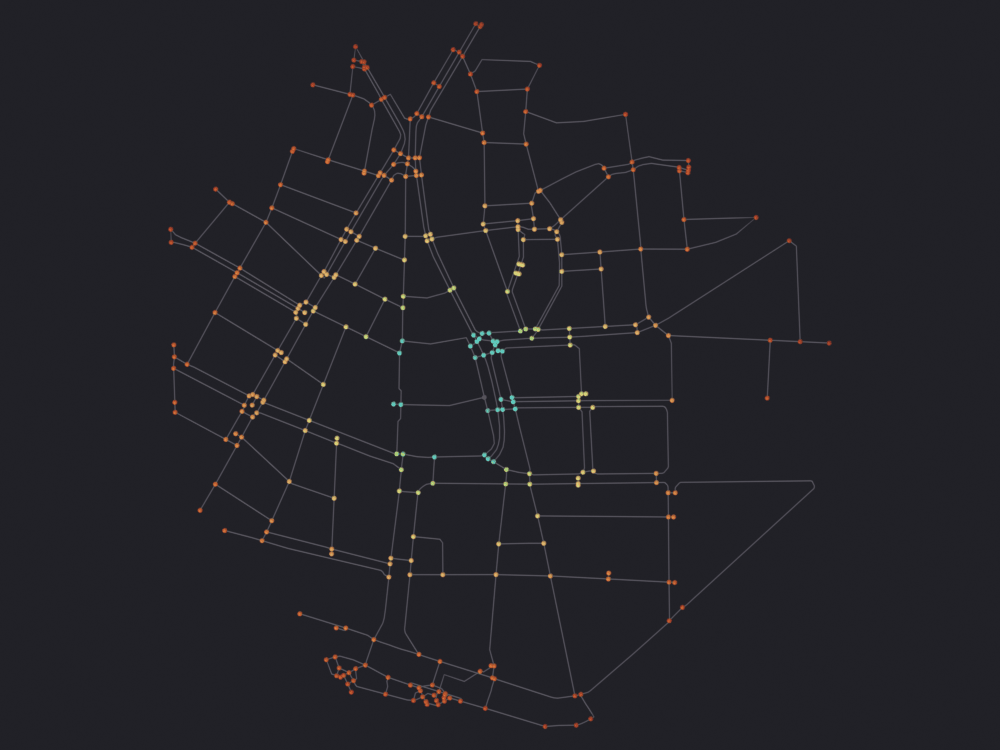
[PASS] 7_catchment.png legible — 4.4% ink (healthy range 0.5–60%)9 · Two caches, and neither of them is the other
| OSMnx response cache | SciGraphs GraphML cache | |
|---|---|---|
| Holds | the raw Overpass JSON | the parsed MultiDiGraph |
| Keyed on | a hash of the query string | <query_name>_<network_type>.graphml |
| Written by | OSMnx, on every request | import_osm_graph, automatically |
| Read by | OSMnx, before every request | get_osmnx_graph, when memory is empty |
| Saves | the network round trip | the parse, and the graph after a restart |
| Set by | ox.settings.cache_folder, via nb.osmnx() |
the osmnx_cache_directory preference |
The first keeps this notebook runnable. The second makes a .blend re-openable: restore_all_graphs_from_cache runs on file load and refills the in-memory dict for every OSMnx object in the scene, so the analysis operators work again without a download.
print("OSMnx response cache")
print(f"  {nb.rel(ox.settings.cache_folder)}")
responses = sorted(CACHE_DIR.glob("*.json"))
print(f"  {len(responses)} responses, "
      f"{sum(p.stat().st_size for p in responses) / 1e6:.1f} MB")

print("\nSciGraphs GraphML cache")
print(f"  {nb.rel(sg_cache.get_cache_directory())}")
entries = sg_cache.list_cached_graphs()
print(f"  {len(entries)} graphs, {sum(e[2] for e in entries):.1f} MB")
for filename, _path, size_mb, _mtime in entries[:6]:
    print(f"    {filename:<48} {size_mb:>6.2f} MB")
if len(entries) > 6:
    print(f"    … and {len(entries) - 6} more")

# `osmnx_view_cached_graphs` is this listing as a dialog, invoke-only, so there
# is nothing to run headless. `osmnx_clear_cache` empties the directory.
print("\ncache operators:",
      sorted(name for name in dir(bpy.ops.scigraphs)
      if "cache" in name and name.startswith("osmnx")))
OSMnx response cache
notebooks/data/cache/osmnx
47 responses, 81.5 MB
SciGraphs GraphML cache
~/.config/blender/5.2/scripts/addons/scigraphs_osmnx_cache
45 graphs, 126.8 MB
39.4699_-0.3763_walk.graphml 1.93 MB
39.4699_-0.3763_drive.graphml 0.63 MB
39.4699_-0.3763_all.graphml 2.04 MB
39.4699_-0.3763_bike.graphml 0.77 MB
polygon_AOI_CiutatVella_drive.graphml 0.18 MB
bbox_39.48_39.46_drive.graphml 0.22 MB
… and 39 more
cache operators: ['osmnx_clear_cache', 'osmnx_delete_cached_graph', 'osmnx_load_from_cache', 'osmnx_open_cache_directory', 'osmnx_save_to_cache', 'osmnx_view_cached_graphs']The GraphML filename is a lossy key, and it collides in silence
The cache entry is named from osmnx_query_name and osmnx_network_type and nothing else (SciGraphs/core/osmnx/cache.py:78-105). For a POINT download osmnx_query_name is f"{lat:.4f}_{lon:.4f}" (data_operators.py:659), so the radius is not in the key, and neither are simplify, retain_all, truncate_by_edge or any custom_filter. Every drive download this notebook made at this center wrote to the same file: the 600 m disc, the unsimplified version, the retain_all=True version. Each overwrote the last, and if get_osmnx_graph ever falls through to disk it gets whichever ran most recently. A BBOX download is keyed on f"bbox_{north:.2f}_{south:.2f}" (data_operators.py:661), dropping east and west entirely: two boxes at the same latitudes are one cache entry.
The in-memory cache is keyed by a UUID per object, so the collision bites only after a restart, or on the load_graph_from_cache fallback.
print(f"query_name for the POINT download  {net.get('osmnx_query_name')!r}")
print(f"cache filename                     "
      f"{sg_cache.generate_cache_filename(net)}")
print(f"the radius that produced it        {RADIUS_M} m, not in the name")

collisions = {}
for obj in bpy.data.objects:
    if obj.get("is_osmnx"):
        collisions.setdefault(
            sg_cache.generate_cache_filename(obj), []).append(obj.name)

print("\nobjects in this scene that share a cache filename:")
shared = {k: v for k, v in collisions.items() if len(v) > 1}
for filename, names in sorted(shared.items()):
    print(f"  {filename:<40} {len(names)}: {', '.join(sorted(names))}")

check("distinct downloads share one cache filename", bool(shared),
      "the radius, simplify and retain_all are all absent from the key")
query_name for the POINT download '39.4699_-0.3763'
cache filename 39.4699_-0.3763_drive.graphml
the radius that produced it 600 m, not in the name
objects in this scene that share a cache filename:
39.4699_-0.3763_drive.graphml 3: Net_drive, Net_drive_raw, Net_point
39.4699_-0.3763_walk.graphml 2: Net_walk, Net_walk_all_components
[PASS] distinct downloads share one cache filename — the radius, simplify and retain_all are all absent from the keyTrueosmnx_save_to_cache
The explicit version of what the import does automatically. It writes the object’s current graph, so it is the way to persist a simplified, consolidated or truncated network, but to the same lossy filename: a consolidated graph would overwrite the raw one at the same center. Give it a distinct osmnx_query_name first; that property is writable and nothing else reads it.
consolidated_obj["osmnx_query_name"] = (
    f"{CENTER[0]:.4f}_{CENTER[1]:.4f}_consolidated{CHOSEN_TOLERANCE}m")
consolidated_obj["osmnx_network_type"] = "drive"
sg.graphs.activate(consolidated_obj)
print("target filename:", sg_cache.generate_cache_filename(consolidated_obj))
print("osmnx_save_to_cache ->", bpy.ops.scigraphs.osmnx_save_to_cache())
written_path = sg_cache.get_cache_filepath(consolidated_obj)
print("written:", pathlib.Path(written_path).name if written_path else None)

check("the consolidated graph has its own cache entry",
      written_path is not None and pathlib.Path(written_path).is_file())
target filename: 39.4699_-0.3763_consolidated20m_drive.graphml
Graph saved to ~/.config/blender/5.2/scripts/addons/scigraphs_osmnx_cache/39.4699_-0.3763_consolidated20m_drive.graphml
Graph cached to: ~/.config/blender/5.2/scripts/addons/scigraphs_osmnx_cache/39.4699_-0.3763_consolidated20m_drive.graphml
Info: Graph cached as: 39.4699_-0.3763_consolidated20m_drive.graphml
osmnx_save_to_cache -> {'FINISHED'}
written: 39.4699_-0.3763_consolidated20m_drive.graphml
[PASS] the consolidated graph has its own cache entryTrue10 · Save
The nodes and edges as a GeoPackage, which keeps the column types GeoJSON loses, plus the tables this notebook measured.
sg.graphs.save_gdf(gdf_nodes, out_dir / "nodes.gpkg")
sg.graphs.save_gdf(gdf_edges, out_dir / "edges.gpkg")

rows = ["method,nodes,edges,length_km"]
for name, obj in methods.items():
    n, m, km = counts(graph_cache.get_osmnx_graph(obj))
    rows.append(f"{name},{n},{m},{km:.2f}")
(out_dir / "download_methods.csv").write_text("\n".join(rows) + "\n",
                                              encoding="utf-8")

rows = ["network_type,nodes,edges,directed_km,street_km"]
for network_type, obj in networks.items():
    n, m, km = counts(graph_cache.get_osmnx_graph(obj))
    rows.append(f"{network_type},{n},{m},{km:.2f},{street_km[network_type]:.2f}")
(out_dir / "network_types.csv").write_text("\n".join(rows) + "\n",
                                           encoding="utf-8")

rows = ["tolerance_m,nodes,edges,median_shift_m,max_shift_m"]
for tolerance, (G_c, _merged, shift) in consolidated.items():
    rows.append(f"{tolerance},{G_c.number_of_nodes()},{G_c.number_of_edges()},"
                f"{np.median(shift):.2f},{shift.max():.2f}")
(out_dir / "consolidation.csv").write_text("\n".join(rows) + "\n",
                                           encoding="utf-8")

print("written to", nb.rel(out_dir))
for entry in sorted(out_dir.iterdir()):
    print(f"  {entry.name:<32} {entry.stat().st_size / 1e3:>9.1f} kB")
written to notebooks/out/10_osmnx
ciutat_vella_drive.graphml 227.3 kB
consolidation.csv 0.1 kB
download_methods.csv 0.1 kB
edges.gpkg 208.9 kB
network_types.csv 0.2 kB
nodes.gpkg 127.0 kB
roundtrip_edges.geojson 200.8 kB
roundtrip_nodes.geojson 50.3 kBRendering
The seven figures are EEVEE through nb.render, top-down and orthographic, look='ink' throughout, each colored by a quantity computed in the cell above it: node_street_count, node_degree, node_merged, node_balance, node_crow_m.
The obvious quantity for section 5 would have been the size of each node’s connected component, and it is unshowable: 98.9 % of the nodes share one value, so every ramp puts the whole network at one stop and the eighteen discarded nodes at the other, where they are eighteen pixels. That tally belongs in a print; the figure went to node_balance instead.
Where a distribution has a long tail, as the merge counts do, the top percentile is clipped with clip_high_pct rather than pinned with vmax. color_graph(vmax=…) sets the property, then scigraphs.color_set_attribute calls update_property_range() and overwrites it with the raw extremes (SciGraphs/ui/coloring/operators.py:374), so a manual range is discarded with nothing to say it happened. The percentile arguments survive.
On Blender’s Vulkan backend, the default on Linux,
gpu.state.point_size_setdoes nothing for the add-on’s shaders, so the SciGraphs GPU engine drawsPOINTandDISKnodes exactly one pixel wide. That engine is not used here, but start Blender with--gpu-backend openglanyway;verify_notebooks.pydoes.
Summary
| Question | Call | What it costs |
|---|---|---|
| Where | osmnx_download_method, five ways, section 1 |
PLACE and ADDRESS cost a geocode as well |
| Which streets | osmnx_network_type |
walk is 6.5x drive here, and all is 7.8x |
| Topology, not centerlines | osmnx_simplify, or simplify=True on download |
they are not the same graph |
| One junction, one node | osmnx_consolidate |
needs a projected, directed graph; nodes move further than the tolerance |
| Undirected / simple | osmnx_to_undirected, osmnx_to_digraph |
the second drops parallel edges for good |
| One connected piece | osmnx_largest_component |
1.1 % of the walk network here, and it is boundary stubs |
| Less than you downloaded | osmnx_truncate_distance / _polygon / _bbox |
the third passes its box in the wrong order, and took this network from 243 nodes to 2 |
| The numbers | osmnx_estimate_area, then osmnx_basic_stats |
the area is a convex hull, not the study area |
| Out and back | graph_to_gdfs / gdfs_to_graph |
loses G.graph, including simplified |
| Out and back, faithfully | osmnx_save_graphml / osmnx_load_graphml |
nothing |
| Not downloading it again | nb.osmnx(), first |
one line, and the notebook runs offline |
Next: 11 · Edge attributes and street orientation, which takes the network built here and asks what its edges are carrying.