import pathlib
import sys
import time


def find_repo():
    """Locate the SciGraphs repository, without relying on the cwd.

    In a normal Jupyter the kernel starts per notebook with the cwd set to its
    folder. Not here: the kernel lives inside Blender and existed before you
    opened anything, so the cwd is wherever Blender was launched from. What the
    extension does know is which folder it is serving to JupyterLab.
    """
    candidates = []
    try:
        import bpy
        prefs = bpy.context.preferences.addons[
            "bl_ext.user_default.jupyter_blender"].preferences
        candidates.append(pathlib.Path(bpy.path.abspath(prefs.notebook_dir)))
    except Exception:
        pass
    candidates.append(pathlib.Path.cwd())

    for base in candidates:
        for directory in (base, *base.parents):
            if (directory / "SciGraphs" / "api" / "graphs.py").is_file():
                return directory

    raise RuntimeError(
        "Cannot find the SciGraphs repository. Point at it by hand:\n"
        "    sys.path.insert(0, '/path/to/SciGraphs-1/notebooks/tools')")


sys.path.insert(0, str(find_repo() / "notebooks" / "tools"))

import bpy
import city2graph as c2g
import geopandas as gpd

# `nb` must import first: it puts this repository on sys.path, so the
# `SciGraphs` import below reads this tree, not the copy Blender installed.
import nb
from nb import check

from SciGraphs import api as sg

ox = nb.osmnx()

CENTER = (39.4699, -0.3763)     # Ciutat Vella, València
RADIUS_M = 700
METRIC_CRS = "EPSG:25830"16 · Proximity graphs
When no flow is observed and no street joins two entities, the relation between them can be posited from geometric closeness. City2Graph offers seven constructions for points and one for polygons, and which you pick is a hypothesis about which spatial relation matters, not a neutral preprocessing step, so the notebook builds all of them over the same points, restaurants and cafés in one neighborhood: knn_graph and fixed_radius_graph for relative and absolute proximity, the four non-parametric constructions (delaunay_graph, gabriel_graph, relative_neighborhood_graph, euclidean_minimum_spanning_tree), the probabilistic waxman_graph, and contiguity_graph for polygons. It closes with the two layer-coupling tools, bridge_nodes and group_nodes.
Two divergences are documented where they appear: generate_proximity_graph reduces polygons to points before calling contiguity_graph(), so CONTIGUITY always yields zero edges, and prox_deduplicate, on by default, rebuilds the GeoDataFrame and loses columns and the original index. The notebook also detects a bug in city2graph 0.3.1 itself: gabriel_graph() compares squared distances against an absolute 1e-12 tolerance, so with UTM coordinates it returns an incorrect graph (248 edges where there should be 453). The check is RNG ⊆ Gabriel, and a workaround is included.
16 · Proximity graphs
When no relation between two entities is observed (no measured flow, no street joining them) it can be postulated from geometric closeness. Choosing among city2graph’s seven constructions for points and one for polygons is not neutral preprocessing: it is a hypothesis about which spatial relation is analytically relevant.
knn_graph: each point to its k nearest neighbors. The ranking matters, the absolute distance does not.fixed_radius_graph: everything inside a threshold, so the radius has physical meaning (a pedestrian catchment, a sensor’s range).delaunay_graph,gabriel_graph,relative_neighborhood_graph,euclidean_minimum_spanning_tree: no k and no radius to choose, the structure comes out of the distribution itself.waxman_graph: probabilistic connection with exponential decay.contiguity_graph: for polygons, Queen or Rook adjacency.
bridge_nodes and group_nodes couple layers.
0 · Setup
1 · The points
Restaurants and cafés. Nodes only: POIs mapped as polygons would be reduced to their centroid, mixing two different things.
pois = ox.features_from_point(
    CENTER, tags={"amenity": ["restaurant", "cafe", "bar"]}, dist=RADIUS_M)
pois = pois[pois.geometry.geom_type == "Point"]
pois = pois.to_crs(METRIC_CRS)[["amenity", "geometry"]].reset_index(drop=True)

print(f"{len(pois)} POIs")
print(pois["amenity"].value_counts().to_string())
check("enough points", len(pois) >= 20, f"{len(pois)}")
462 POIs
amenity
restaurant 301
cafe 115
bar 46
[PASS] enough points — 462TrueAll of these functions need a projected CRS. In degrees, radius=100 is not 100 meters and the results mean nothing.
print("CRS:", pois.crs, "| geographic:", pois.crs.is_geographic)
check("metric CRS", not pois.crs.is_geographic)
CRS: EPSG:25830 | geographic: False
[PASS] metric CRSTrue2 · The seven constructions
The same point cloud, seven different hypotheses about what “near” means.
K = 5
RADIUS = 150.0     # meters

constructions = {
    "knn":       lambda g: c2g.knn_graph(g, k=K),
    "radius":    lambda g: c2g.fixed_radius_graph(g, radius=RADIUS),
    "delaunay":  lambda g: c2g.delaunay_graph(g),
    "gabriel":   lambda g: c2g.gabriel_graph(g),
    "rng":       lambda g: c2g.relative_neighborhood_graph(g),
    "emst":      lambda g: c2g.euclidean_minimum_spanning_tree(g),
    "waxman":    lambda g: c2g.waxman_graph(g, beta=0.5, r0=200.0, seed=42),
}

results = {}
print(f"{'construction':<12} {'nodes':>7} {'edges':>8} {'mean degree':>12} {'s':>6}")
print("-" * 50)
for name, func in constructions.items():
    t0 = time.time()
    nodes, edges = func(pois)
    results[name] = (nodes, edges)
    degree = 2 * len(edges) / len(nodes) if len(nodes) else 0
    print(f"{name:<12} {len(nodes):>7} {len(edges):>8} {degree:>12.2f} "
          f"{time.time() - t0:>6.2f}")
construction nodes edges mean degree s
--------------------------------------------------
knn 462 1418 6.14 0.02
radius 462 6495 28.12 0.06
delaunay 462 1364 5.90 0.02
gabriel 462 476 2.06 0.03
rng 462 550 2.38 0.04
emst 462 461 2.00 0.02
waxman 462 6979 30.21 0.23The EMST is a tree: always n-1 edges, the minimum needed to keep everything connected. Delaunay is the densest of the non-parametric ones, and in theory the four form a chain of subgraphs, EMST ⊆ RNG ⊆ Gabriel ⊆ Delaunay, which is a free integrity test.
def edges_as_set(edges):
    return {tuple(sorted((a, b))) for a, b in edges.index}

edge_sets = {n: edges_as_set(e) for n, (_, e) in results.items()}

check("EMST is a tree",
      len(results["emst"][1]) == len(pois) - 1,
      f"{len(results['emst'][1])} edges for {len(pois)} nodes")
check("EMST ⊆ RNG", edge_sets["emst"] <= edge_sets["rng"])
check("Gabriel ⊆ Delaunay", edge_sets["gabriel"] <= edge_sets["delaunay"])

contained = edge_sets["rng"] <= edge_sets["gabriel"]
print(f"\nRNG ⊆ Gabriel: {contained}  "
      f"(|RNG| = {len(edge_sets['rng'])}, |Gabriel| = {len(edge_sets['gabriel'])}, "
      f"{len(edge_sets['rng'] - edge_sets['gabriel'])} RNG edges are not in Gabriel)")
[PASS] EMST is a tree — 461 edges for 462 nodes
[PASS] EMST ⊆ RNG
[PASS] Gabriel ⊆ Delaunay
RNG ⊆ Gabriel: False (|RNG| = 550, |Gabriel| = 476, 416 RNG edges are not in Gabriel)A real bug in gabriel_graph()
RNG ⊆ Gabriel is a theorem, not a tendency: the RNG lune, the intersection of two discs of radius d(u,v), contains Gabriel’s disc of diameter uv, so the RNG condition is the stricter one. A failed containment means one of the two implementations is wrong. It is gabriel_graph(), in city2graph/proximity.py:911:
tol = 1e-12
...
mask = d2 <= rad2 + tol
if np.count_nonzero(mask) == 2:
An absolute tolerance compared against squared distances. With UTM coordinates (on the order of 4·10⁶ m), d2 is around 10¹³ and float64 leaves an absolute error of ~10⁻³, nine orders of magnitude above the tolerance. Both endpoints also sit exactly on the disc boundary, so count == 2 depends on the noise. False negatives and false positives at once, worse the larger the coordinates, over 250 random points:
| Coordinates | gabriel_graph() |
Correct |
|---|---|---|
| range 0 to 100 | 567 | 567 |
| range 0 to 1000 | 448 | 567 |
| real UTM 30N (725000, 4372000) | 248 | 453 |
A tolerance relative to rad2 reproduces a brute-force check exactly. relative_neighborhood_graph, delaunay_graph and euclidean_minimum_spanning_tree are correct at any scale. Until it is fixed upstream, use RNG instead of Gabriel, or translate the points to the origin first: the result is translation invariant and that recovers much of the precision.
# Translating to the origin is a palliative, not a fix.
pois_centered = pois.copy()
minx, miny, _, _ = pois.total_bounds
pois_centered["geometry"] = pois.geometry.translate(xoff=-minx, yoff=-miny)

_, gabriel_centered = c2g.gabriel_graph(pois_centered)
centered_set = edges_as_set(gabriel_centered)

print(f"Gabriel in UTM coordinates     : {len(edge_sets['gabriel'])} edges")
print(f"Gabriel translated to origin   : {len(centered_set)} edges")
check("translating to the origin restores the RNG ⊆ Gabriel containment",
      edge_sets["rng"] <= centered_set,
      f"{len(edge_sets['rng'] - centered_set)} RNG edges are still outside")
Gabriel in UTM coordinates : 476 edges
Gabriel translated to origin : 832 edges
[PASS] translating to the origin restores the RNG ⊆ Gabriel containment — 0 RNG edges are still outsideTrue3 · The three into the viewport
Each graph in its own collection, offset along X: small multiples in three dimensions.
sg.graphs.clear_scene(keep_anchor=False)
anchor = sg.graphs.anchor(CENTER[0], CENTER[1], scale=0.001, name="Anchor_Proximity")

SEPARATION = 2.2
objects = {}
for i, (name, (nodes, edges)) in enumerate(results.items()):
    obj = sg.graphs.from_gdf(
        nodes, edges, name=f"Prox_{name}", ref=anchor,
        coll="C2G_Proximity",
        markers={"graph_type": name, "k": K, "radius_m": RADIUS})
    if obj is not None:
        obj.location.x += i * SEPARATION
        objects[name] = obj
        print(f"  {obj.name:<18} {obj.get('num_nodes'):>5} nodes, "
              f"{obj.get('num_edges'):>5} edges")

check("the seven graphs are in the scene", len(objects) == 7,
      f"{len(objects)}/7")
Prox_knn 462 nodes, 1418 edges
Prox_radius 462 nodes, 6495 edges
Prox_delaunay 462 nodes, 1364 edges
Prox_gabriel 462 nodes, 476 edges
Prox_rng 462 nodes, 550 edges
Prox_emst 462 nodes, 461 edges
Prox_waxman 462 nodes, 6979 edges
[PASS] the seven graphs are in the scene — 7/7TrueSeven panels of the same point cloud, rendered with EEVEE as in every notebook from 01 onwards. No ground under them: the seven are offset along X and one terrain cannot sit under all of them; buildings arrive in section 5. Straight down through an orthographic camera, render_eevee’s default, with look='ink' and its turbo ramp on a near-black backdrop, shared by notebooks 00 to 07 so their figures compare. The ramp carries edge_weight, the distance in meters of the pair each construction connected.
Turbo is read by hue, not brightness. Over 256 steps its lightness correlates with value at −0.02 against viridis’s +1.00, falling as often as it rises (129 of 255 steps), leaving the order in blue → cyan → green → yellow → red. A tenth of the range costs 19 to 71 units of CIE ΔE (viridis: 13 to 29), and the 0.2 to 0.3 band, holding a seventh of these edges, is stretched hardest.
Each panel is normalized to its own distribution: render_eevee takes vmin/vmax, but the operator underneath re-derives the range from the attribute’s extremes, so an explicit range is silently discarded. Applied afterwards, clip_high_pct does survive, and pulls in the top 2 % so a few long links cannot flatten the rest into the bottom stop.
Blue therefore means “short for this construction”, not “short in meters”. One absolute distance renders 114 ΔE apart at worst across the seven panels under viridis, 128 under turbo; at 50 m, contained by all seven, 67 becomes 154. waxman gains: its 6,979 edges bunch at a third of its own range, close to a single teal, and the share within ΔE 10 of the panel’s median color drops from 15.5 % to 4.9 %, the 0.2 to 0.4 stretch being where turbo spends most of its color. Read the table: EMST and RNG have the lowest medians, radius stops dead at the radius it was given, and waxman is the only one whose maximum reaches the width of the cloud.
print(f"{'construction':<12} {'min':>8} {'median':>8} {'p98':>8} {'max':>9}  (meters)")
print("-" * 52)
for name, (_nodes, edges) in results.items():
    if "weight" not in edges.columns:
        continue
    w = edges["weight"]
    print(f"{name:<12} {w.min():>8.0f} {w.median():>8.0f} "
          f"{w.quantile(0.98):>8.0f} {w.max():>9.0f}")

print("\nedge_weight domain:",
      sg.render.attribute_domain(next(iter(objects.values())), "edge_weight"))

for name, obj in objects.items():
    print(f"{name}: {len(results[name][1])} edges")
    nb.figure(obj, f"renders/02_proximity/1_{name}",
              resolution=(800, 600), width=700,
              look='ink', color_attribute="edge_weight",
              clip_high_pct=98)
construction min median p98 max (meters)
----------------------------------------------------
knn 1 45 173 304
radius 1 99 148 150
delaunay 1 52 223 531
gabriel 5 55 209 280
rng 1 32 152 203
emst 1 28 117 176
waxman 1 233 786 1401
edge_weight domain: EDGE
knn: 1418 edges
Promoted 1 edge attribute(s) to point domain for GN propagation
Info: Geometry Nodes modifier added
Info: Attribute -> edge_weight · edge_weight -> turbo [log] [1.474 … 173.3] on Point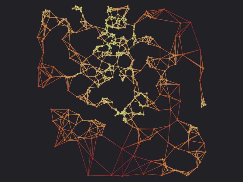
[PASS] 1_knn.png legible — 12.4% ink (healthy range 0.5–60%)
radius: 6495 edges
  Promoted 1 edge attribute(s) to point domain for GN propagation
Info: Geometry Nodes modifier added
Info: Attribute -> edge_weight  ·  edge_weight -> turbo [log]  [1.474 … 148.3] on Point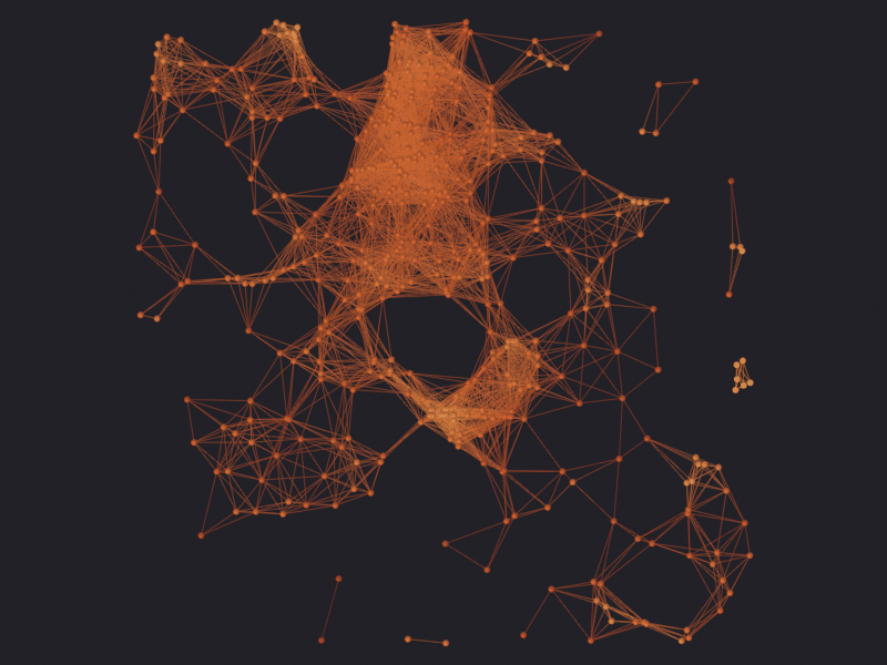
[PASS] 1_radius.png legible — 19.3% ink (healthy range 0.5–60%)
delaunay: 1364 edges
  Promoted 1 edge attribute(s) to point domain for GN propagation
Info: Geometry Nodes modifier added
Info: Attribute -> edge_weight  ·  edge_weight -> turbo [log]  [1.474 … 222.6] on Point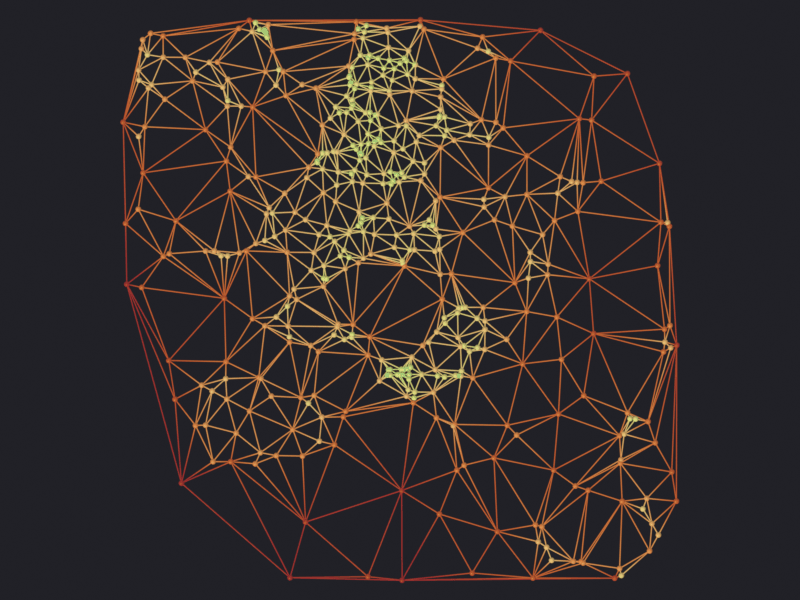
[PASS] 1_delaunay.png legible — 18.2% ink (healthy range 0.5–60%)
gabriel: 476 edges
  Promoted 1 edge attribute(s) to point domain for GN propagation
Info: Geometry Nodes modifier added
Info: Attribute -> edge_weight  ·  edge_weight -> turbo [log]  [4.615 … 208.9] on Point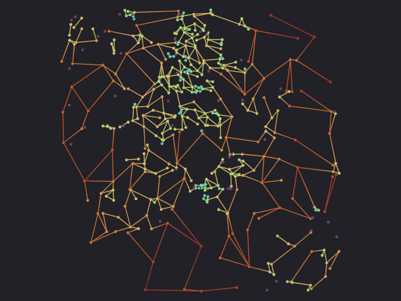
[PASS] 1_gabriel.png legible — 9.4% ink (healthy range 0.5–60%)
rng: 550 edges
  Promoted 1 edge attribute(s) to point domain for GN propagation
Info: Geometry Nodes modifier added
Info: Attribute -> edge_weight  ·  edge_weight -> turbo [log]  [1.474 … 152.2] on Point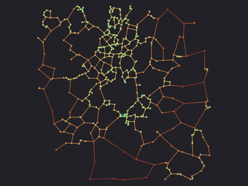
[PASS] 1_rng.png legible — 7.1% ink (healthy range 0.5–60%)
emst: 461 edges
  Promoted 1 edge attribute(s) to point domain for GN propagation
Info: Geometry Nodes modifier added
Info: Attribute -> edge_weight  ·  edge_weight -> turbo [log]  [1.474 … 116.8] on Point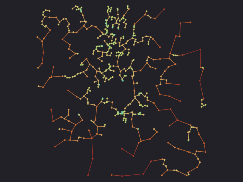
[PASS] 1_emst.png legible — 5.8% ink (healthy range 0.5–60%)
waxman: 6979 edges
  Promoted 1 edge attribute(s) to point domain for GN propagation
Info: Geometry Nodes modifier added
Info: Attribute -> edge_weight  ·  edge_weight -> turbo [log]  [1.474 … 786] on Point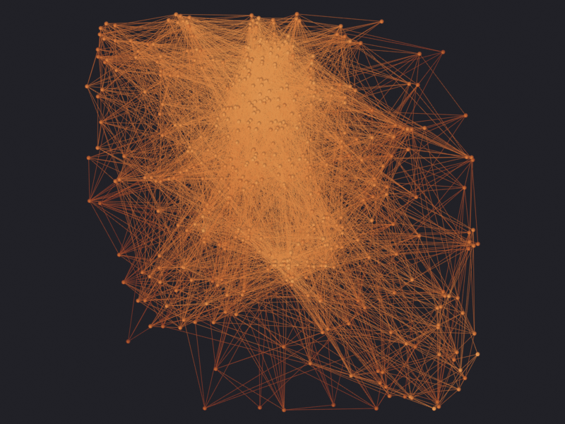
[PASS] 1_waxman.png legible — 43.5% ink (healthy range 0.5–60%)for obj in objects.values():
sg.graphs.visualize(obj, node_size=0.012, edge_thickness=0.002)
sg.graphs.frame()
print("Seven identical clouds, seven different topologies.") Promoted 1 edge attribute(s) to point domain for GN propagation
Info: Geometry Nodes modifier added
Promoted 1 edge attribute(s) to point domain for GN propagation
Info: Geometry Nodes modifier added
Promoted 1 edge attribute(s) to point domain for GN propagation
Info: Geometry Nodes modifier added
Promoted 1 edge attribute(s) to point domain for GN propagation
Info: Geometry Nodes modifier added
Promoted 1 edge attribute(s) to point domain for GN propagation
Info: Geometry Nodes modifier added
Promoted 1 edge attribute(s) to point domain for GN propagation
Info: Geometry Nodes modifier added
Promoted 1 edge attribute(s) to point domain for GN propagation
Info: Geometry Nodes modifier added
Seven identical clouds, seven different topologies.4 · The distance metric is a hypothesis too
The same fixed_radius_graph and radius with Manhattan, Euclidean and network distance give three different graphs. The network one measures along the streets rather than as the crow flies, which is what matters when the threshold stands for a walking time.
G_streets = ox.graph_from_point(CENTER, dist=RADIUS_M, network_type="walk", simplify=True)
_, streets_gdf = ox.graph_to_gdfs(G_streets)
streets_gdf = streets_gdf.to_crs(METRIC_CRS)

metrics = {}
for metric in ("euclidean", "manhattan"):
    nodes, edges = c2g.fixed_radius_graph(pois, radius=RADIUS, distance_metric=metric)
    metrics[metric] = (nodes, edges)

t0 = time.time()
nodes_net, edges_net = c2g.fixed_radius_graph(
    pois, radius=RADIUS, distance_metric="network", network_gdf=streets_gdf)
metrics["network"] = (nodes_net, edges_net)
print(f"network distance computed in {time.time() - t0:.1f} s "
      f"over {len(streets_gdf)} segments")

print()
for metric, (nodes, edges) in metrics.items():
    print(f"  {metric:<11} {len(edges):>6} edges within {RADIUS:.0f} m")
network distance computed in 2.6 s over 5534 segments
euclidean 6495 edges within 150 m
manhattan 4406 edges within 150 m
network 4015 edges within 150 mThe network one always gives fewer or the same: walking the street is never shorter than the straight line, and the difference measures how much the urban fabric distorts real accessibility.
check("network ≤ euclidean",
      len(metrics["network"][1]) <= len(metrics["euclidean"][1]),
      f"{len(metrics['network'][1])} vs {len(metrics['euclidean'][1])}")

for i, (metric, (nodes, edges)) in enumerate(metrics.items()):
    obj = sg.graphs.from_gdf(
        nodes, edges, name=f"Radius_{metric}", ref=anchor,
        coll="C2G_Proximity_Metrics", markers={"distance_metric": metric})
    if obj is not None:
        obj.location.y -= 2.2
        obj.location.x += i * SEPARATION
        sg.graphs.visualize(obj, node_size=0.012, edge_thickness=0.002)
[PASS] network ≤ euclidean — 4015 vs 6495
Promoted 1 edge attribute(s) to point domain for GN propagation
Info: Geometry Nodes modifier added
Promoted 1 edge attribute(s) to point domain for GN propagation
Info: Geometry Nodes modifier added
Promoted 1 edge attribute(s) to point domain for GN propagation
Info: Geometry Nodes modifier added5 · Polygons: contiguity_graph()
For areas the natural relation is not distance but sharing a border. City2Graph wraps libpysal: Queen connects polygons sharing a border or a single vertex, Rook requires a shared border. It is the usual homogeneous reference model for asking what a purely spatial relation buys you, as notebook 18 does.
BLOCKS_RADIUS_M = 400

# Two shapes on purpose: section 5b needs `height` and `building:levels`, which
# only survive on the untrimmed download. From `blocks` alone a skyline could
# only be a constant.
blocks_osm = ox.features_from_point(CENTER, tags={"building": True},
                                    dist=BLOCKS_RADIUS_M)
blocks_osm = blocks_osm[blocks_osm.geometry.geom_type.isin(["Polygon", "MultiPolygon"])]
blocks = blocks_osm.to_crs(METRIC_CRS)[["geometry"]].reset_index(drop=True)
print(f"{len(blocks)} polygons")

nodes_q, edges_q = c2g.contiguity_graph(blocks, contiguity="queen")
nodes_r, edges_r = c2g.contiguity_graph(blocks, contiguity="rook")

print(f"queen {len(edges_q):>6} edges")
print(f"rook  {len(edges_r):>6} edges")
check("Queen contains Rook", len(edges_q) >= len(edges_r))
1022 polygons
queen 1270 edges
rook 1224 edges
[PASS] Queen contains RookTrueThe libpysal warning “The weights matrix is not fully connected: there are N disconnected components” is expected: a set of OSM buildings has blocks that touch no other one, and those are left as isolated components.
The equivalent operator is broken for contiguity.
bpy.ops.scigraphs.generate_proximity_graph()withprox_graph_type = 'CONTIGUITY'extracts the geometry withas_points=True, reducing every polygon to its representative point before callingcontiguity_graph(). Two points never share a border, so it always returns zero edges and raises no error: libpysal only warns about “islands” in the console. Use the direct call in the previous cell. The operator’s other seven constructions do pass the correct geometry.
obj_cont = sg.graphs.from_gdf(
    nodes_q, edges_q, name="Contiguity_Queen", ref=anchor,
    coll="C2G_Proximity_Polygons", markers={"contiguity": "queen"})
print(sg.graphs.summary(obj_cont))

# `contiguity_graph()` has no weight of its own but records the distance
# between the representative points it joined: a long edge crosses a large
# block, a short one is a party wall. The clip earns its place here. Distances
# run 2 m to 90 m, half between 13 and 23 m, and the 26 edges past the 98th
# percentile take the top 55 % of the ramp; clipped, the median moves from 0.17
# of the scale to 0.40.
nb.figure(obj_cont, "renders/02_proximity/2_contiguity_queen",
          look='ink', color_attribute="edge_weight",
          clip_high_pct=98)
{'object': 'Contiguity_Queen', 'type': 'MESH', 'num_nodes': 1022, 'num_edges': 1270, 'is_directed': False, 'vertices': 1022, 'mesh_edges': 1270, 'attributes': ['position', '.edge_verts', '.corner_vert', '.corner_edge', 'node_id', 'edge_weight']}
Promoted 1 edge attribute(s) to point domain for GN propagation
Info: Geometry Nodes modifier added
Info: Attribute -> edge_weight · edge_weight -> turbo [log] [2.323 … 40.22] on Point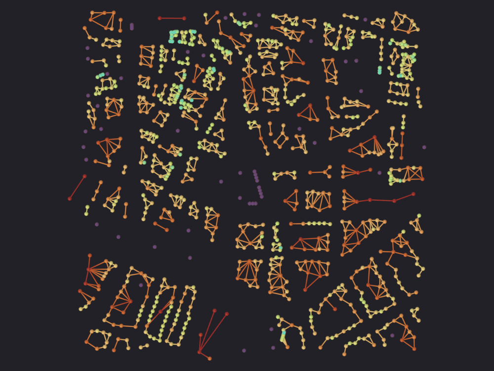
[PASS] 2_contiguity_queen.png legible — 12.9% ink (healthy range 0.5–60%)5b · The same graph over the buildings it is made of
Every node above is a building footprint reduced to its representative point, every edge two of them sharing a border or a corner. Over the extruded footprints it becomes visibly a description of a block.
add_context() builds the ground and the prisms and drops the pair to street level under the graph. It is handed blocks_osm, the tagged download rather than the trimmed analysis copy, so prisms and nodes come from the same polygons.
The radius is padded by seventy percent, for two reasons. features_from_point(dist=400) returns every footprint that intersects a 400 m box, so the polygons run past it and so do this graph’s nodes: ground built at exactly 400 m covers 91 % of it and the graph runs off its own ground. That is what check_alignment() catches, and on a surface it is all it can catch, since a terrain is symmetric about the anchor and so can only be too small, never off-center; buildings carry absolute coordinates and can fail either way. The rest is notebook 13’s framing argument: an orthographic camera framed tight on a square graph in a 4:3 frame needs ground about 1.4 times the graph’s own half-extent. A basemap in the wrong place is what check_alignment() cannot catch, since draping an image moves no vertex; the only test is below, whether the graph runs along the streets in the photograph.
terrain_source="flat"reaches no network. Ciutat Vella has about twenty meters of relief across the frame, under two percent of it; notebook 17 fetches a real DEM over this same center and reports what it got.reference="all". By defaultsettle()measures the ground, putting the graph at street level: right for notebook 17, where the nodes are intersections, wrong here. These nodes are the buildings’ own representative points, so at street level each sits inside a twenty-meter prism and the render is a city with two or three white specks in it.reference="all"measures the tallest roof, so the context drops below the graph.imagery="ESRI_IMAGERY". The claim of the figure is that the nodes are these roofs; on an aerial you can see the courtyards the footprints leave and check that edges cross party walls rather than streets. Zoom 17 costs 36 tiles over a 1.2 km box, under a second cold and a quarter of that from disk, and this box is a little larger; the call prints the count it fetched. Each zoom step quarters or quadruples it, and the fetch refuses above 256 tiles. It also carries a license: the attribution line is printed below and belongs on anything published from this frame.
ctx = sg.context.add_context(obj_cont, CENTER, BLOCKS_RADIUS_M * 1.7, anchor,
                             buildings_gdf=blocks_osm,
                             terrain_source="flat", reference="all",
                             imagery="ESRI_IMAGERY", imagery_zoom=17)
print("real elevation:", ctx["real_elevation"])
print("real imagery  :", ctx["real_imagery"])
sg.context.report(ctx["objects"])
Creating terrain mesh: 2x2 vertices
Terrain mesh created: 4 vertices, 1 faces
flat ground, 1360 x 1360 m (no elevation data)
1022 footprints -> 12538 faces, 23032 vertices
heights: 167 from OSM tags (16.3%), the rest at 21.0 m (median of tagged)
Esri · Satellite (World Imagery): 6x6 = 36 tiles at zoom 17, 1536x1536 px
36 already cached, 0 to fetch (~0.0 MB)
Basemap: ESRI_IMAGERY z=17 → 6×6=36 tiles (1536×1536 px)
Basemap saved: /tmp/scigraphs_basemaps/_composites/basemap_esri_imagery_z17_1787036061.png (1477×1477 px, 0/36 failed tiles)
scigraphs-utils available - Graphviz layouts enabled
Esri · Satellite (World Imagery): 1477x1477 px in 0.3 s (36 tiles from cache)
Tiles © Esri — Source: Esri, Maxar, Earthstar Geographics, and the GIS User Community
context moved -0.08600 Blender units (-86.0 m) so the tallest roof clears z=0 by 1 m
[PASS] Context_Ground aligned with Contiguity_Queen — center off by 0.0143 BU (1.16% of the graph diagonal), covers 100.0% of it, 1.55x its width
[PASS] Context_Buildings aligned with Contiguity_Queen — center off by 0.0332 BU (2.70% of the graph diagonal), covers 100.0% of it, 1.06x its width
real elevation: False
real imagery : True
Context_Ground ground 1.360 x 1.360 x 0.000 BU source=flat real_elevation=False imagery=ESRI_IMAGERY@z17 (36 tiles)
Context_Buildings buildings 0.936 x 0.991 x 0.086 BU 1022 footprints, 16% tagged, default 21.0 m (median of tagged)The credit line. real_imagery above is the only thing worth trusting on whether the photograph arrived: a failed fetch puts the matte material back and says so.
sg.context.attribution(ctx["objects"]) Tiles © Esri — Source: Esri, Maxar, Earthstar Geographics, and the GIS User Community['Tiles © Esri — Source: Esri, Maxar, Earthstar Geographics, and the GIS User Community']With isolate=False every mesh is rendered, and by now that is the seven proximity graphs, the three distance-metric ones and this one, over a grid of X and Y offsets. All but this one step out of the frame by hand.
graphs = [o for o in bpy.data.objects
          if o.type == 'MESH' and "num_nodes" in o.keys()]
for obj in graphs:
    obj.hide_render = obj is not obj_cont

# Ink ceiling lifted for the usual overhead reason (notebook 13): against a
# full-frame aerial the corner pixel is a coin toss. The floor still applies.
path = nb.render(
    obj_cont, "renders/02_proximity/3_contiguity_over_buildings",
    isolate=False, look='ink', color_attribute="edge_weight",
    clip_high_pct=98, verbose=False)
nb.show(path)
nb.check_render(path, maximum=1.0)

for obj in graphs:
    obj.hide_render = False
Promoted 1 edge attribute(s) to point domain for GN propagation
Info: Geometry Nodes modifier added
Info: Attribute -> edge_weight · edge_weight -> turbo [log] [2.323 … 40.22] on Point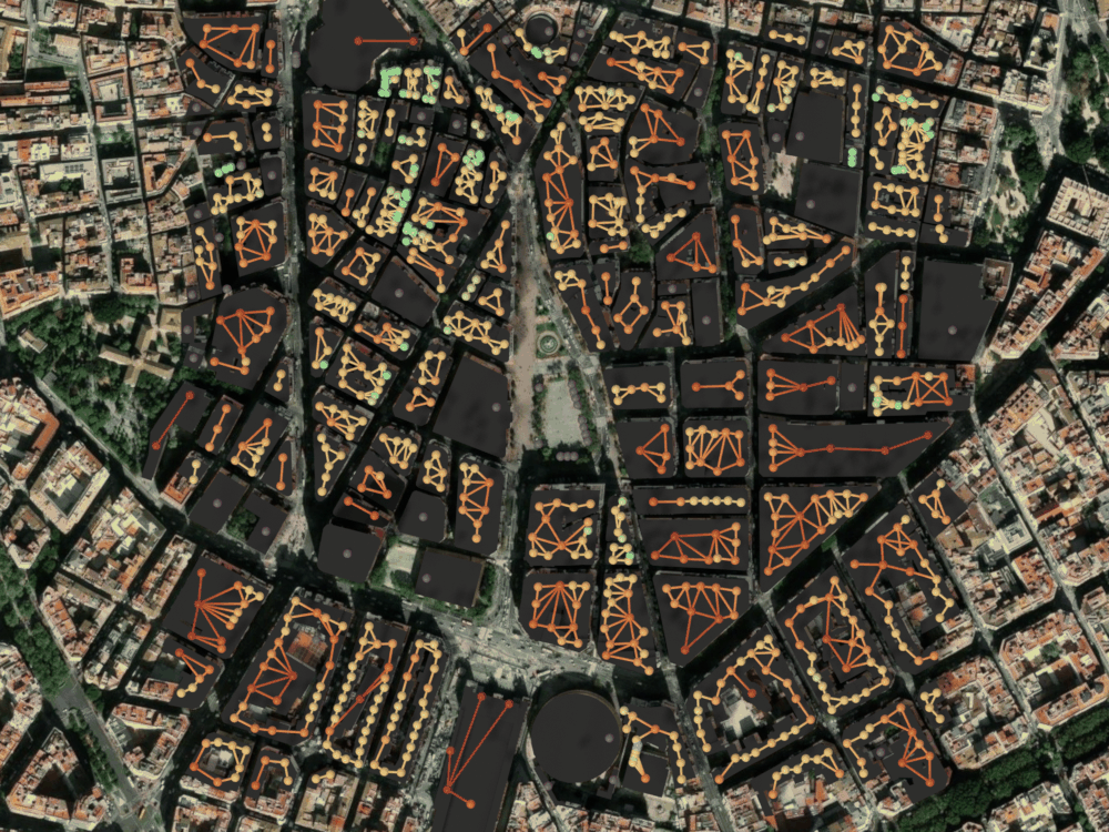
[PASS] 3_contiguity_over_buildings.png legible — 97.9% ink (healthy range 0.5–100%)The offset that lays this graph beside the others is applied afterwards: the context was built about the anchor, and moving the graph away first would leave the two 2.2 Blender units (2.2 km) apart.
if obj_cont is not None:
    obj_cont.location.y += 2.2
    sg.graphs.visualize(obj_cont, node_size=0.01, edge_thickness=0.002)
Promoted 1 edge attribute(s) to point domain for GN propagation
Info: Geometry Nodes modifier added6 · Coupling layers: bridge_nodes()
It generates directed edges between semantic layers, extending kNN and fixed radius across node types, and turns loose layers into a heterogeneous graph. Here: restaurants, cafés and bars, with the is_nearby relations between them.
layers = {
    kind: pois[pois["amenity"] == kind][["geometry"]].reset_index(drop=True)
    for kind in ("restaurant", "cafe", "bar")
}
layers = {k: v for k, v in layers.items() if len(v) >= 3}
for name, gdf in layers.items():
    print(f"  {name:<12} {len(gdf):>4} points")

nodes_dict, edges_dict = c2g.bridge_nodes(layers, proximity_method="knn", k=3)
hetero_summary = nb.describe_hetero(nodes_dict, edges_dict)
restaurant 301 points
cafe 115 points
bar 46 points
nodes
restaurant 301 Point
cafe 115 Point
bar 46 Point
edges
restaurant -> is_nearby -> cafe 903
restaurant -> is_nearby -> bar 903
cafe -> is_nearby -> restaurant 345
cafe -> is_nearby -> bar 345
bar -> is_nearby -> restaurant 138
bar -> is_nearby -> cafe 138The keys of edges_dict are triplets (source_type, relation, target_type). That (a, is_nearby, b) and (b, is_nearby, a) exist separately is not redundancy: the k nearest neighbors are not a symmetric relation.
triplets = list(edges_dict.keys())
print(f"{len(triplets)} relation types")
check("the keys are triplets",
      all(isinstance(t, tuple) and len(t) == 3 for t in triplets))
check("the relation is called is_nearby",
      all(t[1] == "is_nearby" for t in triplets))

obj_bridge = sg.graphs.from_hetero(
    nodes_dict, edges_dict, name="Bridges_POI", ref=anchor,
    coll="C2G_Proximity_Multilayer",
    markers={"graph_type": "bridge_nodes"})
if obj_bridge is not None:
    obj_bridge.location.y += 4.4
    sg.graphs.visualize(obj_bridge, node_size=0.014, edge_thickness=0.002)
    sg.graphs.color_by(obj_bridge, "layer_id", colormap="turbo")
print(sg.graphs.summary(obj_bridge))
# Isolated because section 5b's buildings cover only the inner 400 m and this
# layer cake spans the full 700 m of the POI download.
#
# `layer_id` is a POINT attribute, so the ramp lands on the spheres and leaves
# the bridges neutral. Three categories need separable colors, not a perceptual
# order: turbo's closest pair is 61 ΔE apart, under viridis's 85 but far past
# where two categories merge.
print("layer_id domain:", sg.render.attribute_domain(obj_bridge, "layer_id"))
nb.figure(obj_bridge, "renders/02_proximity/4_bridges_poi",
          look='ink', color_attribute="layer_id")
6 relation types
[PASS] the keys are triplets
[PASS] the relation is called is_nearby
Promoted 2 edge attribute(s) to point domain for GN propagation
Info: Geometry Nodes modifier added
Info: Attribute -> layer_id · layer_id -> turbo [log] [0 … 2] on Point
{'object': 'Bridges_POI', 'type': 'MESH', 'num_nodes': 462, 'num_edges': 2236, 'is_directed': False, 'vertices': 462, 'mesh_edges': 2236, 'attributes': ['position', '.edge_verts', '.corner_vert', '.corner_edge', 'layer_id', 'node_id', 'edge_type_id', 'edge_weight', 'layer_id_color'], 'layer_names': 'restaurant,cafe,bar', 'edge_type_names': 'restaurant_is_nearby_cafe,restaurant_is_nearby_bar,cafe_is_nearby_restaurant,cafe_is_nearby_bar,bar_is_nearby_restaurant,bar_is_nearby_cafe', 'graph_type': 'bridge_nodes'}
layer_id domain: POINT
Promoted 2 edge attribute(s) to point domain for GN propagation
Info: Geometry Nodes modifier added
Info: Attribute -> layer_id · layer_id -> turbo [log] [0 … 2] on Point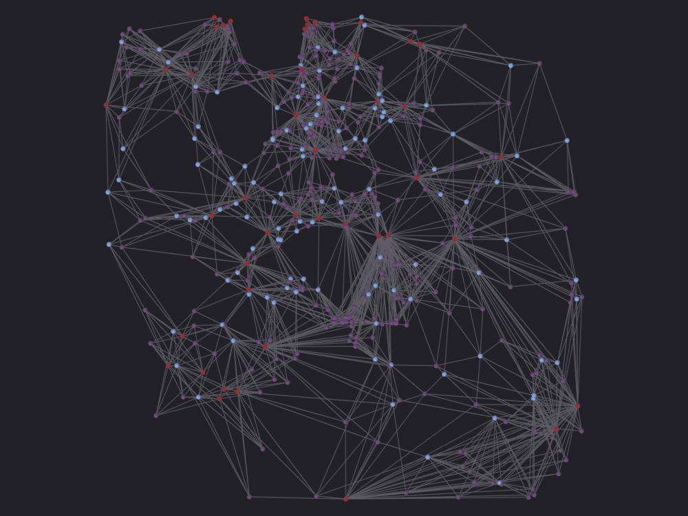
[PASS] 4_bridges_poi.png legible — 22.4% ink (healthy range 0.5–60%)7 · Hierarchy: group_nodes()
The other coupling strategy. Instead of connecting by closeness it nests points inside the polygons that contain them: the membership relation (this stop is in this neighborhood), which moves from the scale of the POI to the census unit.
zones = ox.features_from_point(CENTER, tags={"landuse": True}, dist=RADIUS_M)
zones = zones[zones.geometry.geom_type.isin(["Polygon", "MultiPolygon"])]
zones = zones.to_crs(METRIC_CRS)[["landuse", "geometry"]].reset_index(drop=True)
print(f"{len(zones)} land-use polygons")

if len(zones) >= 2:
    nodes_group, edges_group = c2g.group_nodes(
        zones, pois[["geometry"]], predicate="covered_by")
    nb.describe_hetero(nodes_group, edges_group)

    obj_group = sg.graphs.from_hetero(
        nodes_group, edges_group, name="Grouping_POI_Zone", ref=anchor,
        coll="C2G_Proximity_Groups", markers={"graph_type": "group_nodes"})
    if obj_group is not None:
        obj_group.location.y += 6.6
        sg.graphs.visualize(obj_group, node_size=0.014, edge_thickness=0.002)
    print(sg.graphs.summary(obj_group))
else:
    print("Not enough land-use polygons within this radius; "
          "try another center or a larger radius.")
235 land-use polygons
nodes
polygon 235 Polygon
point 462 Point
edges
polygon -> covers -> point 568
Promoted 2 edge attribute(s) to point domain for GN propagation
Info: Geometry Nodes modifier added
{'object': 'Grouping_POI_Zone', 'type': 'MESH', 'num_nodes': 697, 'num_edges': 568, 'is_directed': False, 'vertices': 697, 'mesh_edges': 568, 'attributes': ['position', '.edge_verts', '.corner_vert', '.corner_edge', 'layer_id', 'node_id', 'edge_type_id', 'edge_weight'], 'layer_names': 'polygon,point', 'edge_type_names': 'polygon_covers_point', 'graph_type': 'group_nodes'}8 · The SciGraphs operator
For the seven point constructions the operator is faithful to city2graph. Load the points as a features object, point prox_feature_object at it, and set the type.
props = bpy.context.scene.city2graph

objs_poi = sg.graphs.from_features(pois, name="POIs_Valencia", ref=anchor,
                                   coll="C2G_Proximity_Operator")
if objs_poi:
    poi_obj = objs_poi[0]
    poi_obj["is_osm_features"] = True
    poi_obj["feature_count"] = len(pois)

    props.prox_feature_object = poi_obj
    props.prox_graph_type = 'KNN'
    props.prox_knn_k = K
    props.prox_distance_metric = 'EUCLIDEAN'
    props.prox_deduplicate = False       # keep the original indices and attributes

    result = bpy.ops.scigraphs.generate_proximity_graph()
    print("generate_proximity_graph ->", result)

    from_operator = [o for o in bpy.data.objects if o.get("is_proximity_graph")]
    for obj in from_operator:
        print(" ", sg.graphs.summary(obj))

    if from_operator:
        direct = len(results["knn"][1])
        via_op = from_operator[0].get("num_edges")
        check("the operator reproduces the direct kNN",
              abs(direct - via_op) <= max(2, direct * 0.02),
              f"direct {direct} vs operator {via_op}")
Using reference projection: center=(39.469900, -0.376300), scale=0.001
Created 1 object(s) from GeoDataFrame with 462 features
Generating KNN graph with metric=euclidean
Deduplication: False, tolerance=0.5m
Loaded cached GeoDataFrame from object: 462 features (Point)
KNN graph created successfully in 0.04s
Info: Generating KNN proximity graph...
Info: Graph generated: 462 nodes, 1418 edges
Info: KNN graph created successfully (0.04s)
generate_proximity_graph -> {'FINISHED'}
{'object': 'KNN_Graph', 'type': 'MESH', 'num_nodes': 462, 'num_edges': 1418, 'is_directed': False, 'vertices': 462, 'mesh_edges': 1418, 'attributes': ['position', '.edge_verts', '.corner_vert', '.corner_edge', 'node_id', 'edge_weight'], 'graph_type': 'KNN'}
[PASS] the operator reproduces the direct kNN — direct 1418 vs operator 1418About
prox_deduplicate. It is on by default and groups near-coincident points by rebuilding the GeoDataFrame asGeoDataFrame(geometry=centroids, crs=...): all non-geometric columns are lost and the original index becomes aRangeIndex. To join the resulting graph back to the source data, turn it off, as the previous cell does.
9 · Saving
output_dir = nb.out("16_proximity")
output_dir.mkdir(parents=True, exist_ok=True)

for name, (nodes, edges) in results.items():
    sg.graphs.save_gdf(edges, output_dir / f"edges_{name}.gpkg")
sg.graphs.save_gdf(pois, output_dir / "pois.gpkg")

print("written to", nb.rel(output_dir))
print(f"  {len(list(output_dir.iterdir()))} files")
written to notebooks/out/16_proximity
8 filesRendering
Every figure comes from EEVEE, through nb.figure(), drawn right after the step that created each object; the PNGs are left in notebooks/out/renders/. Notebook 13 explains how it works and why the geographic notebooks put terrain and extruded buildings under their graphs. Only the contiguity graph gets that treatment here.
The Vulkan warning still applies, to the SciGraphs engine that notebooks 17 and 06 keep for edge sparsification: on Blender’s Vulkan backend (the default on Linux)
gpu.state.point_size_setdoes nothing for the add-on shaders, soPOINTandDISKnodes come out 1 pixel wide. Start Blender with--gpu-backend openglfor any render you intend to look at.
Summary
| Spatial hypothesis | Function | Parameter |
|---|---|---|
| Relative proximity | knn_graph |
k |
| Absolute proximity | fixed_radius_graph |
radius |
| Natural neighborhood | delaunay_graph, gabriel_graph, relative_neighborhood_graph |
none |
| Minimal connectivity | euclidean_minimum_spanning_tree |
none |
| Decay with distance | waxman_graph |
beta, r0 |
| Shared border | contiguity_graph |
queen / rook |
| Coupling between layers | bridge_nodes |
k or radius |
| Hierarchical membership | group_nodes |
predicate |
Next: 05 · Metapaths and the 15-minute city.