Shortest paths, minimum spanning trees, maximum flow and minimum cut, with every claim checked against an answer worked out independently.
The generic algorithm operators never read an edge weight. There is no field for one to travel in, so every weighted branch is guarded by a test that is always false and every edge is worth 1.0. Shortest path reports a hop count as a distance, and deleting the weights from the mesh changes nothing; max-flow and min-cut return 3 = 3 where the answer is 19 = 19.
It also solves a problem the whole suite shares: showing a subset (a path, a tree, a cut) when color cannot carry membership, because an edge attribute is averaged onto the vertices and a two-valued flag lands on the two darkest ends of the ramp. Letting geometry carry membership and color carry magnitude is worth 90 levels of separation for a path, against −15 for the obvious approach.
04 · Paths, spanning trees and flows
Four questions for a weighted graph: cheapest route, cheapest set of edges that keeps it connected, how much flows from source to sink, where the bottleneck is. find_shortest_path, compute_mst, compute_max_flow, compute_min_cut, animate_traversal and animate_flow live in SciGraphs/core/algorithms/ (pathfinding.py, spanning.py, network_flow.py) as thin NetworkX wrappers that read an edge weight if the graph carries one, which on a graph built by the add-on is never. Every operator is silently unweighted; sections 2, 3 and 4 check each against NetworkX in the same cell.
The graphs are abstract and seeded: a weighted lattice, and a hand-built flow network of twelve arcs, small enough that a shortest path is checkable by eye and a min cut of four arcs is countable. Real graphs are notebook 01’s subject, layouts 16’s, centrality and communities 17’s, topological invariants 19’s.
No internet needed.
0 · Setup
import pathlibimport sysdef find_repo():"""Locate the SciGraphs repository, without relying on the cwd. In a normal Jupyter the kernel starts per notebook with the cwd set to its folder. Not here: the kernel lives inside Blender and existed before you opened anything, so the cwd is wherever Blender was launched from. What the extension does know is which folder it is serving to JupyterLab. """ candidates = []try:import bpy prefs = bpy.context.preferences.addons["bl_ext.user_default.jupyter_blender"].preferences candidates.append(pathlib.Path(bpy.path.abspath(prefs.notebook_dir)))exceptException:pass candidates.append(pathlib.Path.cwd())for base in candidates:for directory in (base, *base.parents):if (directory /"SciGraphs"/"api"/"graphs.py").is_file():return directoryraiseRuntimeError("Cannot find the SciGraphs repository. Point at it by hand:\n"" sys.path.insert(0, '/path/to/SciGraphs-1/notebooks/tools')")sys.path.insert(0, str(find_repo() /"notebooks"/"tools"))import bpyimport geopandas as gpdimport networkx as nximport numpy as npimport pandas as pdfrom shapely.geometry import LineString, Point# `nb` must import first: it puts this repository on sys.path, so the# `SciGraphs` import below reads this tree, not the copy Blender installed.import nbfrom nb import checkfrom SciGraphs import api as sgSEED =18rng = np.random.default_rng(SEED)print("networkx", nx.__version__)print("seed", SEED)
networkx 3.6
seed 18
Abstract graphs on a georeferenced pipeline
sg.graphs.from_gdf() wants a nodes GeoDataFrame and an edges GeoDataFrame with a (source, target) MultiIndex (city2graph’s convention), projected through an anchor. There is no abstract entry point, so an abstract graph arrives dressed as a geographic one: positions in a metric CRS, the anchor turning meters into Blender units, CRS and origin canceling out. 200 m spacing at scale=0.001 gives 0.2 Blender units between neighbors, the order the geospatial notebooks work at, so sg.render’s size heuristics land where they were calibrated.
CRS ="EPSG:32630"# UTM 30N; arbitrary, and it cancelsORIGIN = (500000.0, 4600000.0)SPACING =200.0# meters between adjacent lattice nodesdef to_gdfs(graph, coords, edge_attrs=(), node_attrs=None):"""A NetworkX graph as the (nodes, edges) pair `graph_to_blender` wants. `coords` maps node -> (column, row) in lattice units; `edge_attrs` names the edge data keys to carry across, `node_attrs` is a dict of name -> {node: value}. Numeric columns become mesh attributes, prefixed by `geo_mesh`: a node column `depth` lands as `node_depth`, an edge column `weight` as `edge_weight`. That prefix is not cosmetic; see section 1. """def point(n):return (ORIGIN[0] + coords[n][0] * SPACING, ORIGIN[1] + coords[n][1] * SPACING) columns = {} if node_attrs isNoneelse { key: [float(values[n]) for n in graph.nodes()]for key, values in node_attrs.items()} nodes = gpd.GeoDataFrame( columns, geometry=[Point(point(n)) for n in graph.nodes()], index=pd.Index(list(graph.nodes()), name="node"), crs=CRS) rows = []for u, v, data in graph.edges(data=True): row = {"source": u, "target": v,"geometry": LineString([point(u), point(v)])}for key in edge_attrs: row[key] =float(data.get(key, 0.0)) rows.append(row) edges = gpd.GeoDataFrame(rows, crs=CRS).set_index(["source", "target"])return nodes, edges
1 · The test bed: a weighted lattice
A 6×6 four-neighbor lattice, weights drawn once from U(1, 9). Small enough to check every claim against the picture, regular enough that a route deviating from the straight line does so for a visible reason.
SIDE =6G = nx.grid_2d_graph(SIDE, SIDE)G = nx.convert_node_labels_to_integers(G, ordering="sorted", label_attribute="cell")for u, v in G.edges(): G[u][v]["weight"] =float(np.round(rng.uniform(1.0, 9.0), 2))CELL = {n: c for n, c in G.nodes(data="cell")}print(f"nodes {G.number_of_nodes()} edges {G.number_of_edges()}")weights = np.array([d["weight"] for _, _, d in G.edges(data=True)])print(f"weights min {weights.min():.2f} median {np.median(weights):.2f} "f"max {weights.max():.2f}")check("the lattice is connected", nx.is_connected(G))check("every edge carries a weight",all("weight"in d for _, _, d in G.edges(data=True)))
nodes 36  edges 60
weights  min 1.06  median 5.41  max 8.76
[PASS] the lattice is connected
[PASS] every edge carries a weight
{'object': 'Lattice', 'type': 'MESH', 'num_nodes': 36, 'num_edges': 60, 'is_directed': False, 'vertices': 36, 'mesh_edges': 60, 'attributes': ['position', '.edge_verts', '.corner_vert', '.corner_edge', 'node_id', 'edge_weight'], 'graph_type': 'grid_2d_graph'}

attributes:
  position                     POINT   FLOAT_VECTOR
  .edge_verts                  EDGE    INT32_2D
  .corner_vert                 CORNER  INT
  .corner_edge                 CORNER  INT
  node_id                      POINT   INT
  edge_weight                  EDGE    FLOAT
The prefix.weight in the GeoDataFrame is edge_weight on the mesh (geo_mesh.py:300). Anything looking a weight up by its source name finds nothing and falls back to a default; that already produced a GPU edge backbone silently ranked by mesh order.
mesh = obj_grid.datastored = np.zeros(len(mesh.edges), dtype=np.float64)mesh.attributes["edge_weight"].data.foreach_get("value", stored)pairs = np.empty(len(mesh.edges) *2, dtype=np.int32)mesh.edges.foreach_get("vertices", pairs)pairs = pairs.reshape(-1, 2)source_order = np.array([G[int(a)][int(b)]["weight"] for a, b in pairs])check("the weight column arrives as edge_weight, not weight","edge_weight"in mesh.attributes and"weight"notin mesh.attributes)check("edge_weight is on the EDGE domain", sg.render.attribute_domain(obj_grid, "edge_weight") =="EDGE")check("edge_weight is aligned with the mesh edge order", np.allclose(stored, source_order),f"max deviation {np.abs(stored - source_order).max():.3g}")
[PASS] the weight column arrives as edge_weight, not weight
[PASS] edge_weight is on the EDGE domain
[PASS] edge_weight is aligned with the mesh edge order — max deviation 3.43e-07
True
A weight on the mesh is not safe there
Applying a layout zeroes every EDGE-domain attribute. Layout operators end by calling geometry.rebuild_edges(obj) (ui/operators/scigraphs/layout_operators.py:322, :397, :483, :589, :639; also data_operators.py:41), which deletes every bmesh edge and rebuilds it from the edges_data string (core/mesh/geometry.py:1227-1248). Topology comes back identical, edge attributes at zero: same names, same length, no values. Point attributes survive; the vertices are never rebuilt.
Nothing raises. A shortest path over all-zero weights is still a path, an MST still a tree, a max flow over all-zero capacities 0. Only the last looks wrong. The demonstration below runs on a throwaway copy.
scratch_nodes, scratch_edges = to_gdfs(G, CELL, edge_attrs=("weight",), node_attrs={"tag": {n: float(n)for n in G.nodes()}})scratch = sg.graphs.from_gdf(scratch_nodes, scratch_edges, name="Scratch", ref=ANCHOR, coll="Algo")def edge_values(obj, attribute):"""An EDGE-domain attribute as an array, or None when it is not there.""" attr = obj.data.attributes.get(attribute)if attr isNoneor attr.domain !='EDGE':returnNone values = np.zeros(len(obj.data.edges)) attr.data.foreach_get("value", values)return valuesdef node_values(obj, attribute):"""The POINT counterpart of `edge_values`.""" attr = obj.data.attributes.get(attribute)if attr isNoneor attr.domain !='POINT':returnNone values = np.zeros(len(obj.data.vertices)) attr.data.foreach_get("value", values)return valuesbefore_edges = edge_values(scratch, "edge_weight")before_nodes = node_values(scratch, "node_tag")sg.graphs.activate(scratch)# `SPRING` reaches `nx.spring_layout` with no `seed=`# (`core/mesh/layouts/networkx_layouts.py:8` and `:18`), so seeding NumPy's# global generator immediately before the call is the only way to pin it.np.random.seed(SEED)print("apply_layout ->", bpy.ops.scigraphs.apply_layout(algorithm='SPRING', iterations=30, scale=5.0))after_edges = edge_values(scratch, "edge_weight")after_nodes = node_values(scratch, "node_tag")print(f"\n mesh edges {len(before_edges)} → {len(after_edges)}")print(f" edge_weight range {before_edges.min():.2f}-{before_edges.max():.2f}"f" → {after_edges.min():.2f}-{after_edges.max():.2f}")print(f" node_tag range {before_nodes.min():.0f}-{before_nodes.max():.0f}"f" → {after_nodes.min():.0f}-{after_nodes.max():.0f}")check("the layout kept the topology", len(after_edges) ==len(before_edges))check("the layout kept the point attribute", np.allclose(before_nodes, after_nodes))check("the layout zeroed the edge attribute, silently", np.count_nonzero(after_edges) ==0,"the attribute is still on the mesh, and every value is 0.0")sg.graphs.activate(scratch)bpy.context.scene.scigraphs.pathfinding_source ="0"bpy.context.scene.scigraphs.pathfinding_target ="35"bpy.ops.scigraphs.find_shortest_path()check("and the algorithms answer anyway","shortest_path"in scratch.data.attributes,f"a path of {scratch['shortest_path_nodes']} nodes, distance "f"{scratch['shortest_path_length']:.2f}, over weights that are ""all zero")bpy.data.objects.remove(scratch, do_unlink=True)
======================================================================
Layout algorithm: SPRING
Graph: 36 nodes, 60 edges
Parameters:
  - algorithm: SPRING
  - iterations: 30
  - scale: 5.0000
  - num_nodes: 36
  - num_edges: 60
Execution time: 0.002s
Status: success
======================================================================

Info: Layout 'SPRING' applied
apply_layout -> {'FINISHED'}

  mesh edges          60 → 60
  edge_weight range   1.06-8.76 → 0.00-0.00
  node_tag range      0-35 → 0-35
[PASS] the layout kept the topology
[PASS] the layout kept the point attribute
[PASS] the layout zeroed the edge attribute, silently — the attribute is still on the mesh, and every value is 0.0
Info: Path found: 11 nodes, distance: 10.00
[PASS] and the algorithms answer anyway — a path of 11 nodes, distance 10.00, over weights that are all zero
The rule, here and for anything computing on edge values: lay the graph out first, or not at all, and write the edge attributes last. Every graph here has its positions decided by construction, so no layout operator touches an object that survives this cell. weights_intact() checks that before each of the four algorithms. None of the operators reads these values, but the mesh is the record a later reader will trust.
def weights_intact(obj, attribute, reference, label):"""Assert an edge attribute still holds the values it was built with.""" values = edge_values(obj, attribute)if values isNone:return check(f"{label}: {attribute} survives", False, "gone")return check(f"{label}: {attribute} survives",len(values) ==len(reference)and np.allclose(values, reference)and np.count_nonzero(values) ==len(values),f"{len(values)} values, "f"{values.min():.2f}-{values.max():.2f}, none zero")weights_intact(obj_grid, "edge_weight", stored, "test bed")
[PASS] test bed: edge_weight survives — 60 values, 1.06-8.76, none zero
True
The first figure, and what it is really showing
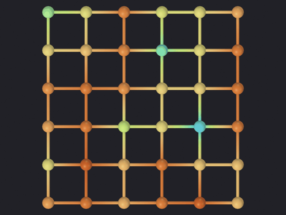
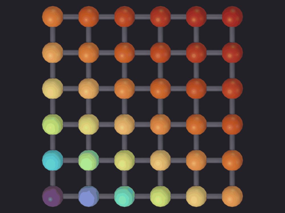
The house style, once. Every figure is EEVEE through nb.figure(), top-down orthographic (a map read at an angle cannot be measured off the page), look='ink', the blackest of the five looks, with turbo, whose low stop is a dark blue rather than a black that would swallow a thin tube. Color always from an attribute computed here, node size always from the graph. Here the attribute is edge_weight, and the figure exposes something everything after it works around.
NODE_FRACTION =0.16# see the Rendering section: 0.35 buries this latticenb.figure(obj_grid, "renders/04_algorithms/1_lattice", look='ink', color_attribute="edge_weight", node_fraction=NODE_FRACTION)
  Promoted 1 edge attribute(s) to point domain for GN propagation
Info: Geometry Nodes modifier added
Info: Attribute -> edge_weight  ·  edge_weight -> turbo [log]  [1.06 … 8.76] on Point
[PASS] 1_lattice.png legible — 15.9% ink (healthy range 0.5–60%)
Each tube is a gradient, not one color: no edge is drawn in the color of its own weight. A Blender color attribute may only live on POINT or CORNER (core/coloring/attributes.py:144), and CORNER needs faces, which a graph mesh has none of, so an EDGE-domain attribute is written to POINT by averaging the incident edges at every vertex (core/coloring/attributes.py:227). That averaging decides how a subset of edges can be drawn at all, so it is worth measuring.
degree = np.zeros(len(mesh.vertices))totals = np.zeros(len(mesh.vertices))for (a, b), w inzip(pairs, stored):for v in (a, b): totals[v] += w degree[v] +=1expected = totals / np.maximum(degree, 1)layer = obj_grid.data.color_attributes[0]print(f"color layer '{layer.name}' domain {layer.domain} "f"type {layer.data_type}")check("the color layer is on POINT, not EDGE", layer.domain =="POINT")check("one color per vertex, not one per edge",len(layer.data) ==len(mesh.vertices),f"{len(layer.data)} colors, {len(mesh.vertices)} vertices, "f"{len(mesh.edges)} edges")# A vertex whose mean matches none of its incident weights cannot be showing# any edge's value, whatever the shader does with it later.incident_weights = [stored[[i for i, (a, b) inenumerate(pairs) if v in (a, b)]]for v inrange(len(mesh.vertices))]mismatched = [v for v, w inenumerate(incident_weights)iflen(w) >1andnot np.any(np.isclose(w, expected[v]))]check("no vertex is showing an edge's own value",len(mismatched) ==len( [w for w in incident_weights iflen(w) >1]),f"{len(mismatched)} of {len(mesh.vertices)} vertices")print(f"\nper-vertex mean of incident edge_weight: "f"{expected.min():.2f} … {expected.max():.2f}")print(f"per-edge edge_weight : "f"{stored.min():.2f} … {stored.max():.2f}")print("the ramp is fitted to the second range and painted with the first")
color layer 'edge_weight_color'  domain POINT  type FLOAT_COLOR
[PASS] the color layer is on POINT, not EDGE
[PASS] one color per vertex, not one per edge — 36 colors, 36 vertices, 60 edges
[PASS] no vertex is showing an edge's own value — 36 of 36 vertices

per-vertex mean of incident edge_weight: 1.84 … 7.07
per-edge edge_weight                  : 1.06 … 8.76
the ramp is fitted to the second range and painted with the first
2 · Shortest paths
NetworkX on the same graph is the reference: once counting hops, once summing weight.
SOURCE, TARGET =0, 35# opposite corners of the latticehop_path = nx.shortest_path(G, SOURCE, TARGET)hop_len = nx.shortest_path_length(G, SOURCE, TARGET)weighted_path = nx.shortest_path(G, SOURCE, TARGET, weight="weight")weighted_len = nx.shortest_path_length(G, SOURCE, TARGET, weight="weight")def cost_of(path):returnsum(G[a][b]["weight"] for a, b inzip(path, path[1:]))print(f"unweighted {hop_len} hops cost {cost_of(hop_path):6.2f}{hop_path}")print(f"weighted {len(weighted_path) -1} hops "f"cost {weighted_len:6.2f}{weighted_path}")check("the two routes are not the same", hop_path != weighted_path)check("the weighted route is cheaper by weight", weighted_len < cost_of(hop_path),f"{weighted_len:.2f} against {cost_of(hop_path):.2f}")check("the unweighted route is not longer in hops", hop_len <=len(weighted_path) -1)
unweighted  10 hops   cost  43.11   [0, 1, 2, 3, 4, 5, 11, 17, 23, 29, 35]
weighted    10 hops   cost  31.26   [0, 6, 12, 13, 14, 20, 21, 22, 28, 29, 35]
[PASS] the two routes are not the same
[PASS] the weighted route is cheaper by weight — 31.26 against 43.11
[PASS] the unweighted route is not longer in hops
True
Both routes take 10 hops, as every monotone staircase from one corner to the other does. The weight decides which staircase, and the gap in cost is the size of the mistake an unweighted answer makes.
What the operator does
bpy.ops.scigraphs.find_shortest_path() reads pathfinding_source, pathfinding_target and pathfinding_algorithm, and nothing else. There is no field for a weight attribute anywhere in the property group (properties/splitter_properties.py:387-409).
weights_intact(obj_grid, "edge_weight", stored, "before find_shortest_path")sg.graphs.activate(obj_grid)props = bpy.context.scene.scigraphsprops.pathfinding_source =str(SOURCE)props.pathfinding_target =str(TARGET)props.pathfinding_algorithm ='DIJKSTRA'result = bpy.ops.scigraphs.find_shortest_path()print("find_shortest_path ->", result)print(f" nodes on the path : {obj_grid['shortest_path_nodes']}")print(f" reported distance : {obj_grid['shortest_path_length']}")flag = np.zeros(len(mesh.vertices))mesh.attributes["shortest_path"].data.foreach_get("value", flag)operator_path =sorted(int(i) for i in np.flatnonzero(flag >0.5))print(f" path (as a node set): {operator_path}")check("the operator's distance is the hop count, not the weighted cost",abs(obj_grid["shortest_path_length"] - hop_len) <1e-6andabs(obj_grid["shortest_path_length"] - weighted_len) >1.0,f"{obj_grid['shortest_path_length']:.2f} = {hop_len} hops, "f"not {weighted_len:.2f}")
[PASS] before find_shortest_path: edge_weight survives — 60 values, 1.06-8.76, none zero
Info: Path found: 11 nodes, distance: 10.00
find_shortest_path -> {'FINISHED'}
  nodes on the path : 11
  reported distance : 10.0
  path (as a node set): [0, 6, 12, 13, 14, 15, 16, 17, 23, 29, 35]
[PASS] the operator's distance is the hop count, not the weighted cost — 10.00 = 10 hops, not 31.26
True
The weight is never read.parse_graph_data() builds a GraphData(nodes, edges, None) (core/mesh/mesh_utils.py:100); GraphData has only nodes, edges, dataframe (core/algorithms/graph.py:3). Every algorithm guards its weight lookup with hasattr(graph_data, 'edge_weights') (pathfinding.py:32, spanning.py:29, network_flow.py:31), an attribute no object the add-on constructs has, so the guard is False everywhere and the weight is the literal 1.0. The operator is breadth-first search wearing Dijkstra’s name.
Strip edge_weight off the mesh entirely and run it again.
backup = stored.copy()mesh.attributes.remove(mesh.attributes["edge_weight"])print("edge_weight on the mesh:", "edge_weight"in mesh.attributes)bpy.ops.scigraphs.find_shortest_path()flag_without = np.zeros(len(mesh.vertices))mesh.attributes["shortest_path"].data.foreach_get("value", flag_without)check("removing the weight changes nothing", np.array_equal(flag, flag_without)andabs(obj_grid["shortest_path_length"] - hop_len) <1e-6,"same path, same reported distance")restored = mesh.attributes.new(name="edge_weight", type='FLOAT', domain='EDGE')restored.data.foreach_set("value", backup.tolist())print("edge_weight restored:", "edge_weight"in mesh.attributes)weights_intact(obj_grid, "edge_weight", stored, "after the experiment")
edge_weight on the mesh: False
Info: Path found: 11 nodes, distance: 10.00
[PASS] removing the weight changes nothing — same path, same reported distance
edge_weight restored: True
[PASS] after the experiment: edge_weight survives — 60 values, 1.06-8.76, none zero
True
Two failure modes look identical from here: the weight is never read (this one, and no state on the object would show it), or the weight is read after a layout has wiped it to zero. weights_intact() catches the second; nothing catches the first except comparing against a computation done elsewhere.
ASTAR is the same: a_star_path() takes the node positions for its heuristic and the same 1.0 for weights (pathfinding.py:87). BELLMAN_FORD is in the enum but never dispatched; the operator tests for 'ASTAR' and sends the rest to Dijkstra (ui/operators/scigraphs/algorithms_operators.py:151).
The route out, taken for all four algorithms: compute with NetworkX, write the answer back as an attribute, and let the operators put it into the scene, which they do faithfully.
props.pathfinding_algorithm ='ASTAR'bpy.ops.scigraphs.find_shortest_path()print(f"A* distance {obj_grid['shortest_path_length']:.2f}")props.pathfinding_algorithm ='BELLMAN_FORD'bpy.ops.scigraphs.find_shortest_path()print(f"Bellman-Ford (→ Dijkstra) distance "f"{obj_grid['shortest_path_length']:.2f}")props.pathfinding_algorithm ='DIJKSTRA'check("all three menu entries report the same unweighted distance",abs(obj_grid["shortest_path_length"] - hop_len) <1e-6)
Info: Path found: 11 nodes, distance: 10.00
A*        distance 10.00
Info: Path found: 11 nodes, distance: 10.00
Bellman-Ford (→ Dijkstra) distance 10.00
[PASS] all three menu entries report the same unweighted distance
True
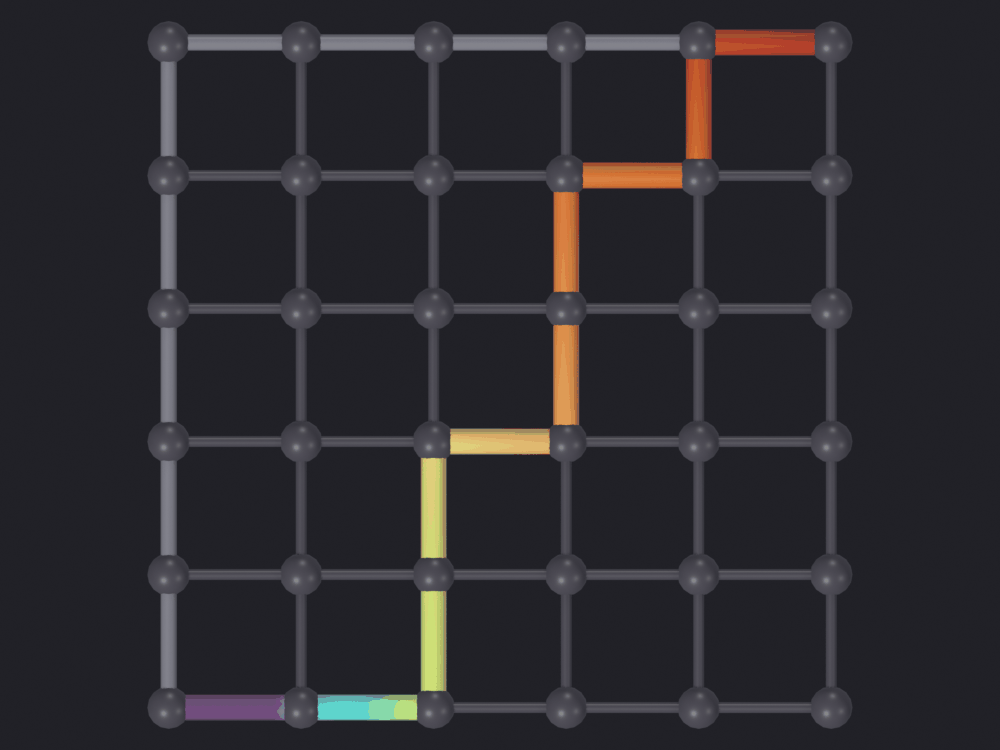
Drawing a path
A path is a subset of the edges, not a continuous attribute. The Rendering section measures why color cannot carry membership here; geometry carries it instead, and overlay() is that arrangement: a second graph object drawn thicker over a context drawn darker, which leaves color for a magnitude.
CONTEXT = (0.085, 0.080, 0.100) # measured in the Rendering sectionFAT =2.4# highlight tube radius, relative to contextLAYERS = [obj_grid] # every graph object, for hide bookkeepingdef plain(obj):"""Strip a previous coloring so a flat `color=` decides the object again. `sg.render.material()` never takes a material away and `geometry_nodes()` re-wires whichever color shader it finds, both so that a graph colored and then rendered keeps its colormap. The context object wants the opposite and has to ask for it. """ layers = obj.data.color_attributesfor name in [a.name for a in layers]: layers.remove(layers[name])for key in ("scigraphs_last_color_attribute", "scigraphs_color_attr"):if key in obj.keys():del obj[key] obj.data.materials.clear()return objdef luminance(path):"""(rgb, luminance) for a PNG, on the 0-255 scale it was written in."""from PIL import Image rgb = np.asarray(Image.open(str(path)).convert("RGB"), dtype=np.float32)return rgb, 0.2126* rgb[..., 0] +0.7152* rgb[..., 1] +0.0722* rgb[..., 2]def overlay(base, highlight, attribute, filename, extra=(), node_fraction=NODE_FRACTION, fat=FAT, measure=True, context_color=CONTEXT):"""Draw `highlight` over `base`, and measure whether it reads. Returns the render's path and, when `measure`, the median luminance of the pixels the highlight reaches (found by rendering the same frame again with it hidden) against the median of the context's own ink. """ sizes = sg.render.autoscale_geometry(base, node_fraction=node_fraction, verbose=False)for obj, ratio, color in [(highlight, fat, context_color), *extra]: sg.render.autoscale_geometry(obj, node_fraction=node_fraction, verbose=False) obj["scigraphs_node_size"] = sizes["node_radius"] *1e-3 obj["scigraphs_edge_thickness"] = sizes["edge_radius"] * ratio sg.render.material(obj, color=color) sg.render.geometry_nodes(obj)# `nodes_only` defaults True for a point attribute. These spheres were# just shrunk to nothing, so the colormap has to reach the tubes: measured# on the tree figure, 70 levels of separation against 16. sg.render.color_graph(highlight, attribute, colormap="turbo", nodes_only=False, verbose=False) shown = {base, highlight, *(o for o, _, _ in extra)} hidden = [o for o in LAYERS if o notin shown] plain(base)# `shrink_png` picks its palette per image, so a pair compared pixel by# pixel stays unquantized until after the measurement. full = nb.render( base, filename, look='ink', isolate=False, color=context_color, node_fraction=node_fraction, hide=hidden, verbose=False, shrink=not measure)ifnot measure: plain(base)return full, None reference = nb.render( base, filename +"_context", look='ink', isolate=False, color=context_color, node_fraction=node_fraction, hide=hidden + [highlight], verbose=False, shrink=False) rgb_full, lum_full = luminance(full) rgb_ref, lum_ref = luminance(reference) reached = np.abs(lum_full - lum_ref) >8 ink_ref = np.abs(rgb_ref - rgb_ref.reshape(-1, 3)[0]).sum(axis=2) >24 numbers = {"highlight_median": float(np.median(lum_full[reached])),"highlight_p05": float(np.percentile(lum_full[reached], 5)),"highlight_area": float(reached.mean()),"context_median": float(np.median(lum_ref[ink_ref])), } numbers["separation"] = numbers["highlight_median"] - numbers["context_median"] plain(base) sg.preview.shrink_png(full) sg.preview.shrink_png(reference)return full, numbers
The highlight carries the cumulative cost from the source on the node domain: 0 at the start, the total at the end. Being a point attribute, it escapes section 1’s averaging, and each tube interpolates two genuinely adjacent costs. The unweighted route goes underneath in flat mid gray: three tiers, lattice, hop route, weighted route.
Info: Geometry Nodes modifier added
Info: Geometry Nodes modifier added
Info: Attribute -> node_cost  ·  node_cost -> turbo [log]  [0 … 31.26] on Point
  Promoted 1 edge attribute(s) to point domain for GN propagation
Info: Geometry Nodes modifier added
  Promoted 1 edge attribute(s) to point domain for GN propagation
Info: Geometry Nodes modifier added
[PASS] 2_paths.png legible — 17.6% ink (healthy range 0.5–60%)
  weighted route : median luminance 136, dimmest 5% at 67
  lattice        : median luminance 75
  separation     : 61 gray levels
3 · Minimum spanning trees
The cheapest set of edges that leaves the graph connected: 35 out of 60 on this 36-node lattice, so the missing edges are what to look for.
The claim “this is a minimum spanning tree” has four parts and none implies the others. Notebook 16 checks its proximity graphs the same way, by containment rather than count.
tree = nx.minimum_spanning_tree(G, weight="weight")tree_weight =sum(d["weight"] for _, _, d in tree.edges(data=True))check("n − 1 edges", tree.number_of_edges() == G.number_of_nodes() -1,f"{tree.number_of_edges()} for {G.number_of_nodes()} nodes")check("acyclic", nx.is_forest(tree))check("spanning: one component, every node in it", nx.is_connected(tree)andset(tree.nodes()) ==set(G.nodes()))check("a subgraph of the lattice, not a new graph", {tuple(sorted(e)) for e in tree.edges()}<= {tuple(sorted(e)) for e in G.edges()})print(f"\nMST weight {tree_weight:.2f} "f"against {weights.sum():.2f} for the whole lattice")
[PASS] n − 1 edges — 35 for 36 nodes
[PASS] acyclic
[PASS] spanning: one component, every node in it
[PASS] a subgraph of the lattice, not a new graph

MST weight 119.10 against 297.73 for the whole lattice
Minimality is the one claim a structural check cannot make. Sampling random spanning trees is enough to catch an implementation that returns a tree instead of the tree, which is the failure mode below.
TRIALS =200sampled = []for _ inrange(TRIALS): perturbed = nx.Graph() perturbed.add_nodes_from(G.nodes())for u, v in G.edges(): perturbed.add_edge(u, v, key=float(rng.random())) random_tree = nx.minimum_spanning_tree(perturbed, weight="key") sampled.append(sum(G[u][v]["weight"] for u, v in random_tree.edges()))sampled = np.array(sampled)check("no sampled spanning tree beats it",bool((sampled >= tree_weight -1e-9).all()),f"{TRIALS} random spanning trees, cheapest {sampled.min():.2f}, "f"median {np.median(sampled):.2f}, against {tree_weight:.2f}")
[PASS] no sampled spanning tree beats it — 200 random spanning trees, cheapest 149.67, median 175.71, against 119.10
True
What the operator does
weights_intact(obj_grid, "edge_weight", stored, "before compute_mst")sg.graphs.activate(obj_grid)props.spanning_algorithm ='KRUSKAL'print("compute_mst ->", bpy.ops.scigraphs.compute_mst())print(f" edges {obj_grid['mst_edges']}")print(f" weight {obj_grid['mst_weight']}")check("the operator finds the right number of edges", obj_grid["mst_edges"] == G.number_of_nodes() -1)check("its weight is the edge count, not the sum of the weights",abs(obj_grid["mst_weight"] - (G.number_of_nodes() -1)) <1e-6,f"{obj_grid['mst_weight']:.2f} = 35 × 1.0, not {tree_weight:.2f}")kruskal_edges = {tuple(sorted(e)) for e in nx.minimum_spanning_tree( nx.Graph([(u, v, {"w": 1.0}) for u, v in G.edges()]), algorithm="kruskal", weight="w").edges()}kruskal_cost =sum(G[u][v]["weight"] for u, v in kruskal_edges)print(f"the tree the operator actually returned costs {kruskal_cost:.2f}")print(f"the minimum spanning tree costs {tree_weight:.2f}")print(f"the median of {TRIALS} random spanning trees "f"{np.median(sampled):.2f}")check("what the operator returned is a spanning tree",len(kruskal_edges) == G.number_of_nodes() -1)check("and it is not the minimum one", kruskal_cost > tree_weight +1e-9,f"{kruskal_cost - tree_weight:.2f} more, "f"{(kruskal_cost / tree_weight -1) *100:.0f}% over")
[PASS] before compute_mst: edge_weight survives — 60 values, 1.06-8.76, none zero
Info: Kruskal: 35 edges, weight: 35.00
compute_mst -> {'FINISHED'}
  edges  35
  weight 35.0
[PASS] the operator finds the right number of edges
[PASS] its weight is the edge count, not the sum of the weights — 35.00 = 35 × 1.0, not 119.10
the tree the operator actually returned costs 174.36
the minimum spanning tree costs             119.10
the median of 200 random spanning trees    175.71
[PASS] what the operator returned is a spanning tree
[PASS] and it is not the minimum one — 55.26 more, 46% over
True
Same cause as section 2, different symptom. With every weight equal to 1 every spanning tree is minimal, so Kruskal returns whichever it reaches first: a valid tree at a real cost the operator never computes, priced above outside Blender. Nothing in the add-on can tell you the gap is there.
The result does not reach the mesh either.spanning.py builds an edge_in_mst array, one flag per edge in mesh order, exactly what a figure needs (spanning.py:42-48); SCIGRAPHS_OT_ComputeMST.execute keeps num_edges and total_weight and drops it (ui/operators/scigraphs/algorithms_operators.py:210).
print("attributes after compute_mst:")print(" ", [a.name for a in mesh.attributes])check("no per-edge MST attribute was written",notany(a.name.startswith("mst") or a.name =="edge_in_mst"for a in mesh.attributes))
attributes after compute_mst:
  ['position', '.edge_verts', '.corner_vert', '.corner_edge', 'node_id', 'shortest_path', 'edge_weight']
[PASS] no per-edge MST attribute was written
True
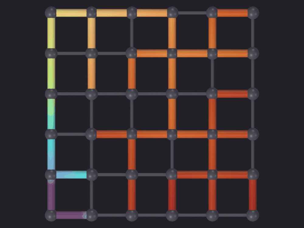
The tree, drawn
The highlight carries depth in the tree from node 0, a point attribute again: distance from the root along the tree’s own edges, so the ramp reads outward from the root rather than across the frame.
depth = nx.single_source_shortest_path_length(tree, SOURCE)tree_graph = nx.Graph()tree_graph.add_nodes_from(G.nodes())tree_graph.add_edges_from(tree.edges())nodes_t, edges_t = to_gdfs(tree_graph, CELL, node_attrs={"depth": {n: float(depth[n])for n in G.nodes()}})obj_tree = sg.graphs.from_gdf(nodes_t, edges_t, name="MST", ref=ANCHOR, coll="Algo")LAYERS.append(obj_tree)print(f"tree depth from node {SOURCE}: 0 … {max(depth.values())}")path, mst_numbers = overlay(obj_grid, obj_tree, "node_depth","renders/04_algorithms/3_mst")nb.show(path)nb.check_render(path)print(f" tree : median luminance {mst_numbers['highlight_median']:.0f}, "f"{mst_numbers['highlight_area'] *100:.1f}% of the frame")print(f" lattice : median luminance {mst_numbers['context_median']:.0f}")print(f" separation: {mst_numbers['separation']:.0f} gray levels")
tree depth from node 0: 0 … 15
Info: Geometry Nodes modifier added
Info: Attribute -> node_depth  ·  node_depth -> turbo [log]  [0 … 15] on Point
  Promoted 1 edge attribute(s) to point domain for GN propagation
Info: Geometry Nodes modifier added
  Promoted 1 edge attribute(s) to point domain for GN propagation
Info: Geometry Nodes modifier added
[PASS] 3_mst.png legible — 21.9% ink (healthy range 0.5–60%)
  tree    : median luminance 109, 12.3% of the frame
  lattice : median luminance 74
  separation: 35 gray levels
4 · Max-flow and min-cut
These two are one theorem: the maximum flow from a source to a sink equals the total capacity of the cheapest set of arcs whose removal disconnects them. It is the one claim that fails loudly when either half is wrong, so it is checked numerically here.
A lattice would be a bad demonstration, its cuts uninteresting and its capacities invented anyway. This is a hand-built network of eight nodes and twelve arcs, laid out left to right in layers, with capacities chosen so the min cut is not simply the arcs leaving the source or entering the sink. It crosses two layers, which is what makes it worth drawing.
CAPACITY = { (0, 1): 20, (0, 2): 6, (0, 3): 8, (1, 4): 3, (1, 5): 2, (2, 4): 3, (2, 5): 5, (3, 5): 2, (3, 6): 7, (4, 7): 14, (5, 7): 12, (6, 7): 10,}LAYOUT = {0: (0.0, 1.5), 1: (1.4, 3.0), 2: (1.4, 1.5), 3: (1.4, 0.0),4: (2.8, 3.0), 5: (2.8, 1.5), 6: (2.8, 0.0), 7: (4.2, 1.5)}SRC, SINK =0, 7F = nx.DiGraph()for (u, v), c in CAPACITY.items(): F.add_edge(u, v, capacity=float(c))print(f"nodes {F.number_of_nodes()} arcs {F.number_of_edges()} "f"source {SRC} → sink {SINK}")print(f"capacity leaving the source : "f"{sum(c for (u, _), c in CAPACITY.items() if u == SRC)}")print(f"capacity entering the sink : "f"{sum(c for (_, v), c in CAPACITY.items() if v == SINK)}")
flow_value, flow_dict = nx.maximum_flow(F, SRC, SINK, capacity="capacity")cut_value, (near, far) = nx.minimum_cut(F, SRC, SINK, capacity="capacity")cut_edges =sorted((u, v) for u in near for v in far if F.has_edge(u, v))for u, v in F.edges(): F[u][v]["flow"] =float(flow_dict[u][v])print(f"max flow {flow_value:.0f}")print(f"min cut {cut_value:.0f} over {len(cut_edges)} arcs {cut_edges}")print(f"source side {sorted(near)} sink side {sorted(far)}")check("max flow = min cut", abs(flow_value - cut_value) <1e-9,f"{flow_value:.0f} = {cut_value:.0f}")check("the cut's capacity is that number",abs(sum(CAPACITY[e] for e in cut_edges) - cut_value) <1e-9," + ".join(str(CAPACITY[e]) for e in cut_edges)+f" = {cut_value:.0f}")check("every cut arc is saturated",all(abs(F[u][v]["flow"] - CAPACITY[(u, v)]) <1e-9for u, v in cut_edges))check("flow is conserved at every intermediate node",all(abs(sum(flow_dict[w][x] for x in F.successors(w))-sum(flow_dict[x][w] for x in F.predecessors(w))) <1e-9for w in F.nodes() if w notin (SRC, SINK)))check("the cut crosses more than one layer",len({u for u, _ in cut_edges}) >1,f"it leaves nodes {sorted({u for u, _ in cut_edges})}")
max flow  19
min cut   19  over 4 arcs [(0, 2), (0, 3), (1, 4), (1, 5)]
source side [0, 1]   sink side [2, 3, 4, 5, 6, 7]
[PASS] max flow = min cut — 19 = 19
[PASS] the cut's capacity is that number — 6 + 8 + 3 + 2 = 19
[PASS] every cut arc is saturated
[PASS] flow is conserved at every intermediate node
[PASS] the cut crosses more than one layer — it leaves nodes [0, 1]
True
Into Blender, and the first thing the operators say
graph_to_blender hard-codes is_directed = False on everything it builds (core/mesh/geo_mesh.py:249); the edges frame’s directedness is never consulted. Both flow operators refuse an undirected graph, so they reject a directed graph imported this way.
nodes_f, edges_f = to_gdfs(F, LAYOUT, edge_attrs=("capacity", "flow"))obj_flow = sg.graphs.from_gdf(nodes_f, edges_f, name="FlowNetwork", ref=ANCHOR, coll="Algo", markers={"graph_type": "flow_network"})LAYERS.append(obj_flow)print(sg.graphs.summary(obj_flow))capacities = np.array([CAPACITY[(u, v)] for u, v in F.edges()])weights_intact(obj_flow, "edge_capacity", capacities,"before compute_max_flow")sg.graphs.activate(obj_flow)props.flow_source =str(SRC)props.flow_sink =str(SINK)try: bpy.ops.scigraphs.compute_max_flow() refused =NoneexceptRuntimeErroras exc: refused =str(exc)print("compute_max_flow on the graph as built:", refused)check("a directed graph arrives marked undirected", obj_flow.get("is_directed") isFalseand refused isnotNone)
{'object': 'FlowNetwork', 'type': 'MESH', 'num_nodes': 8, 'num_edges': 12, 'is_directed': False, 'vertices': 8, 'mesh_edges': 12, 'attributes': ['position', '.edge_verts', '.corner_vert', '.corner_edge', 'node_id', 'edge_capacity', 'edge_flow'], 'graph_type': 'flow_network'}
[PASS] before compute_max_flow: edge_capacity survives — 12 values, 2.00-20.00, none zero
Error: Max flow requires directed graph
compute_max_flow on the graph as built: Error: Max flow requires directed graph

[PASS] a directed graph arrives marked undirected
True
The marker is a custom property, so the workaround is one line. A workaround, not a fix: the arcs survived the import in the right order, only the flag is wrong.
obj_flow["is_directed"] =Trueprint("compute_max_flow ->", bpy.ops.scigraphs.compute_max_flow())print("compute_min_cut ->", bpy.ops.scigraphs.compute_min_cut())operator_flow =float(obj_flow["max_flow_value"])operator_cut =float(obj_flow["min_cut_value"])print(f"\n operator max flow {operator_flow:.0f} min cut {operator_cut:.0f}")print(f" networkx max flow {flow_value:.0f} min cut {cut_value:.0f}")partition = np.zeros(len(obj_flow.data.vertices))obj_flow.data.attributes["min_cut_partition"].data.foreach_get("value", partition)operator_near =sorted(int(i) for i in np.flatnonzero(partition >0.5))print(f" operator source side {operator_near}")print(f" networkx source side {sorted(near)}")
Info: Max flow computed: 3.00
compute_max_flow -> {'FINISHED'}
Info: Min cut: 3.00, 3 edges
compute_min_cut  -> {'FINISHED'}

  operator max flow 3   min cut 3
  networkx max flow 19   min cut 19
  operator source side [0, 1, 2, 3, 4, 5, 6]
  networkx source side [0, 1]
The duality holds, on a different question. With every capacity read as 1.0 the network is an arc-counting problem whose answer is 3, the three arcs into the sink. max_flow == min_cut is still true on that unit-capacity graph, so the two numbers agreeing with each other is no evidence that they agree with the data.
Most of the operator is correct: the topology, the direction of every arc, the source and sink, and min_cut_partition, which really is the reachable set of the residual graph, of the unit-capacity network.
unit = nx.DiGraph()for u, v in F.edges(): unit.add_edge(u, v, capacity=1.0)unit_flow, _ = nx.maximum_flow(unit, SRC, SINK, capacity="capacity")unit_cut, (unit_near, _) = nx.minimum_cut(unit, SRC, SINK, capacity="capacity")check("the operators solve the unit-capacity network exactly",abs(operator_flow - unit_flow) <1e-9andabs(operator_cut - unit_cut) <1e-9and operator_near ==sorted(unit_near),f"{operator_flow:.0f} = {unit_flow:.0f}, and the same partition")check("the operators' own duality holds",abs(operator_flow - operator_cut) <1e-9)check("and it is the wrong network",abs(operator_flow - flow_value) >1e-9,f"{operator_flow:.0f} against {flow_value:.0f}")
[PASS] the operators solve the unit-capacity network exactly — 3 = 3, and the same partition
[PASS] the operators' own duality holds
[PASS] and it is the wrong network — 3 against 19
True
network_flow.py also computes an edge_flow array (network_flow.py:41-47) and an edge_in_cut array (network_flow.py:104-110), and the operators keep neither: ComputeMaxFlow stores one float (algorithms_operators.py:246) and ComputeMinCut stores the node partition and one float (algorithms_operators.py:288-293). The per-arc answer, the drawable half of a flow solution, is discarded in both.
The flow itself
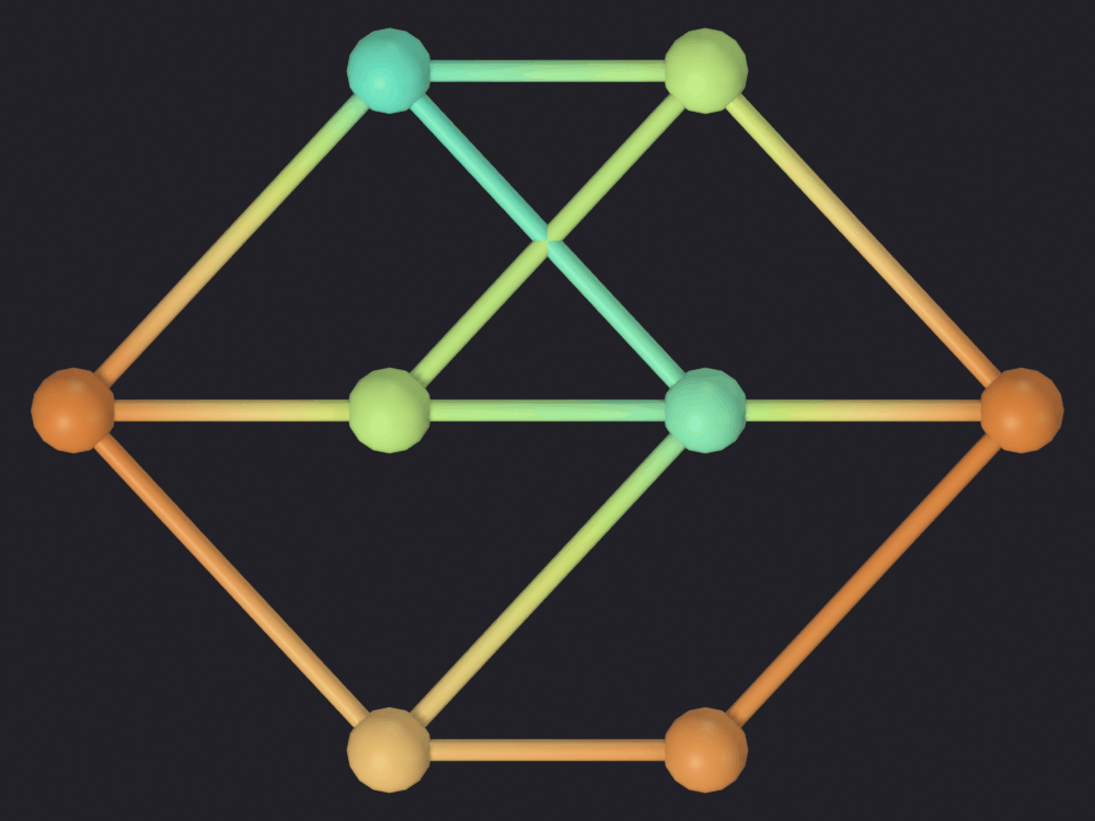
edge_flow here is the real solution, written back from NetworkX: continuous and on every arc, so a plain single-object figure, with section 1’s caveat that the tube gradients are the per-vertex averaging rather than arcs disagreeing with themselves.
The figure cannot show direction. Geometry Nodes draws a tube per edge with no arrowhead, so which way an arc points is in the printed list below and nowhere in the picture.
print("arc capacity flow")for (u, v), c in CAPACITY.items(): bar ="#"*int(round(F[u][v]["flow"]))print(f" {u} → {v}{c:8.0f}{F[u][v]['flow']:4.0f}{bar}")nb.figure(obj_flow, "renders/04_algorithms/4_flow", look='ink', color_attribute="edge_flow", node_fraction=0.22)
[PASS] 4_flow.png legible — 14.9% ink (healthy range 0.5–60%)
The cut, drawn as a set of arcs
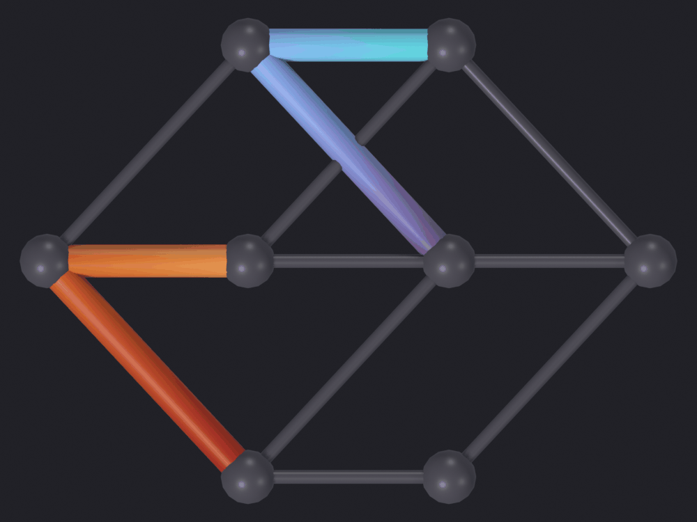
Same arrangement as the path and the tree: the four cut arcs as their own object, thicker, over the network drawn dark. They carry their capacity, the four numbers whose sum is the max flow.
The endpoint problem from the Rendering section bites hardest here, and the numbers below say by how much: with only four values in the highlight, the smallest and the largest sit on turbo’s two ends, both among its darkest stops.
cut_graph = nx.DiGraph()cut_graph.add_nodes_from(F.nodes())for u, v in cut_edges: cut_graph.add_edge(u, v, capacity=float(CAPACITY[(u, v)]))nodes_c, edges_c = to_gdfs(cut_graph, LAYOUT, edge_attrs=("capacity",))obj_cut = sg.graphs.from_gdf(nodes_c, edges_c, name="MinCut", ref=ANCHOR, coll="Algo")LAYERS.append(obj_cut)path, cut_numbers = overlay(obj_flow, obj_cut, "edge_capacity","renders/04_algorithms/5_min_cut", node_fraction=0.22)nb.show(path)nb.check_render(path)print(f" cut : median luminance {cut_numbers['highlight_median']:.0f}, "f"dimmest 5% at {cut_numbers['highlight_p05']:.0f}")print(f" network : median luminance {cut_numbers['context_median']:.0f}")print(f" separation: {cut_numbers['separation']:.0f} gray levels "f"(the tree's was {mst_numbers['separation']:.0f})")
  Promoted 1 edge attribute(s) to point domain for GN propagation
Info: Geometry Nodes modifier added
Info: Attribute -> edge_capacity  ·  edge_capacity -> turbo [log]  [2 … 8] on Point
  Promoted 2 edge attribute(s) to point domain for GN propagation
Info: Geometry Nodes modifier added
  Promoted 2 edge attribute(s) to point domain for GN propagation
Info: Geometry Nodes modifier added
[PASS] 5_min_cut.png legible — 18.5% ink (healthy range 0.5–60%)
  cut     : median luminance 126, dimmest 5% at 69
  network : median luminance 74
  separation: 52 gray levels (the tree's was 35)
edge_capacity is on the EDGE domain, so section 1’s averaging applies. A cut is close to a matching, though, and on a matching the average of the incident edges at a vertex is the edge’s own value: four of the six endpoints here carry exactly one cut arc and are exact; the two the cut leaves twice show the average of their pair.
incident = {}for u, v in cut_edges: incident.setdefault(u, []).append(CAPACITY[(u, v)]) incident.setdefault(v, []).append(CAPACITY[(u, v)])exact = [n for n, caps in incident.items() iflen(caps) ==1]print(f"endpoints touched by exactly one cut arc: {sorted(exact)} "f"({len(exact)} of {len(incident)})")for n, caps insorted(incident.items()):print(f" node {n}: {caps} → drawn as {sum(caps) /len(caps):.1f}")
endpoints touched by exactly one cut arc: [2, 3, 4, 5] (4 of 6)
  node 0: [6, 8] → drawn as 7.0
  node 1: [3, 2] → drawn as 2.5
  node 2: [6] → drawn as 6.0
  node 3: [8] → drawn as 8.0
  node 4: [3] → drawn as 3.0
  node 5: [2] → drawn as 2.0
5 · Traversal and flow animation
animate_traversal and animate_flow produce animation: keyframes on a custom property, plus a frame_change_post handler that recomputes an activation attribute as the timeline moves. A mid-animation frame is a threshold on a number, and the number is the thing, so neither is a figure here.
The quantity underneath is renderable. Both operators compute a per-node ordering before they touch the timeline and write it to the mesh: traversal_order (BFS or DFS visit index) and flow_distance (steps from the nearest source). Ordinary point attributes, and the figure below is one.
sg.graphs.activate(obj_grid)props.traversal_algorithm ='BFS'props.traversal_start_mode ='MANUAL'props.traversal_start_nodes =str(SOURCE)props.traversal_animation_loop =Falseprops.traversal_animation_speed =30frame_end_before = bpy.context.scene.frame_endprint("animate_traversal ->", bpy.ops.scigraphs.animate_traversal())order = np.zeros(len(mesh.vertices))mesh.attributes["traversal_order"].data.foreach_get("value", order)print(f" visited {obj_grid['traversal_visited_count']} nodes")print(f" order {order.min():.0f} … {order.max():.0f}")print(f" keyframes {obj_grid.animation_data isnotNone}")print(f" frame_end {frame_end_before} → {bpy.context.scene.frame_end}")print(f" handlers "f"{[h.__name__for h in bpy.app.handlers.frame_change_post]}")reference_order = {n: i for i, n inenumerate(nx.bfs_tree(G, SOURCE).nodes())}check("every node was visited", obj_grid["traversal_visited_count"] == G.number_of_nodes())check("the order is a permutation of 0 … n−1",sorted(order.astype(int)) ==list(range(G.number_of_nodes())))check("it agrees with a NetworkX BFS from the same root",all(order[n] == reference_order[n] for n in G.nodes()))
Info: BFS animation: 30 frames, 36 nodes
animate_traversal -> {'FINISHED'}
  visited      36 nodes
  order        0 … 35
  keyframes    True
  frame_end    250 → 31
  handlers     ['update_traversal_activation']
[PASS] every node was visited
[PASS] the order is a permutation of 0 … n−1
[PASS] it agrees with a NetworkX BFS from the same root
True
What is thrown away.analysis.calculate_bfs_traversal returns order, depth and parent (core/algorithms/analysis.py:582-593) and the operator writes only order (algorithms_operators.py:53-56). depth is the BFS layer, the unweighted distance from the root, and parent is the BFS tree. Both are more useful than the visit index and neither reaches the mesh.
The visit index is still a legitimate figure: a total order where the depth is only partial, and on a lattice from one corner the two agree on the shape. The wavefront in the picture is the BFS layer structure.
  Promoted 1 edge attribute(s) to point domain for GN propagation
Info: Geometry Nodes modifier added
Info: Attribute -> traversal_order  ·  traversal_order -> turbo [log]  [0 … 35] on Point
[PASS] 6_traversal.png legible — 29.9% ink (healthy range 0.5–60%)
Flow animation, as numbers
animate_flow needs a directed graph and gives the propagation distance from the nodes with no incoming arcs. Here that is one node, the source, so the distances are arc-count layers from a BFS, not the max-flow solution the name suggests.
sg.graphs.activate(obj_flow)props.flow_animation_loop =Falseprops.flow_animation_speed =25print("animate_flow ->", bpy.ops.scigraphs.animate_flow())distance = np.zeros(len(obj_flow.data.vertices))obj_flow.data.attributes["flow_distance"].data.foreach_get("value", distance)layers_nx = nx.single_source_shortest_path_length(F, SRC)print("node flow_distance BFS layer flow out")for n insorted(F.nodes()): out =sum(F[n][x]["flow"] for x in F.successors(n))print(f" {n}{distance[n]:.0f}{layers_nx[n]}"f" {out:.0f}")check("flow_distance is the arc-count layer, not anything about flow",all(distance[n] == layers_nx[n] for n in F.nodes()))check("and it is unrelated to the flow each node carries", distance[1] == distance[2] == distance[3]andlen({sum(F[n][x]["flow"] for x in F.successors(n))for n in (1, 2, 3)}) >1,"nodes 1, 2 and 3 share a layer and carry different flow")
Info: Flow animation created: 25 frames (single pass)
animate_flow -> {'FINISHED'}
node  flow_distance  BFS layer  flow out
  0        0          0        19
  1        1          1        5
  2        1          1        6
  3        1          1        8
  4        2          2        6
  5        2          2        7
  6        2          2        6
  7        3          3        0
[PASS] flow_distance is the arc-count layer, not anything about flow
[PASS] and it is unrelated to the flow each node carries — nodes 1, 2 and 3 share a layer and carry different flow
True
Cleaning up after an animation
Both operators leave state that outlives the cell: keyframes on the object, a shortened frame_end, and a handler in bpy.app.handlers.frame_change_post that rewrites an attribute on every frame change. Under the shared kernel that would be the next notebook’s problem, so this one puts it back.
for obj in (obj_grid, obj_flow): obj.animation_data_clear()for handler inlist(bpy.app.handlers.frame_change_post):if handler.__name__in ("update_traversal_activation","update_flow_activation"): bpy.app.handlers.frame_change_post.remove(handler)bpy.context.scene.frame_end = frame_end_beforebpy.context.scene.frame_set(bpy.context.scene.frame_start)check("no keyframes left", obj_grid.animation_data isNoneand obj_flow.animation_data isNone)check("no frame-change handlers left",not [h for h in bpy.app.handlers.frame_change_postif h.__name__.startswith("update_")],f"{[h.__name__for h in bpy.app.handlers.frame_change_post]}")check("the timeline is back", bpy.context.scene.frame_end == frame_end_before)
[PASS] no keyframes left
[PASS] no frame-change handlers left — []
[PASS] the timeline is back
True
6 · Save
The four answers as tables, so they can be checked without Blender.
out_dir = nb.out("18_algorithms")out_dir.mkdir(parents=True, exist_ok=True)pd.DataFrame( [{"source": u, "target": v, "weight": d["weight"],"in_mst": int(tuple(sorted((u, v))) in {tuple(sorted(e))for e in tree.edges()}),"on_weighted_path": int((u, v) inset(zip(weighted_path, weighted_path[1:]))or (v, u) inset(zip(weighted_path, weighted_path[1:]))),"on_hop_path": int((u, v) inset(zip(hop_path, hop_path[1:]))or (v, u) inset(zip(hop_path, hop_path[1:])))}for u, v, d in G.edges(data=True)]).to_csv(out_dir /"lattice_edges.csv", index=False)pd.DataFrame( [{"source": u, "target": v, "capacity": CAPACITY[(u, v)],"flow": F[u][v]["flow"], "in_min_cut": int((u, v) inset(cut_edges))}for u, v in F.edges()]).to_csv(out_dir /"flow_arcs.csv", index=False)pd.DataFrame([ {"question": "shortest path", "networkx": round(weighted_len, 2),"operator": round(float(obj_grid["shortest_path_length"]), 2),"what the operator solved": "hop count"}, {"question": "minimum spanning tree", "networkx": round(tree_weight, 2),"operator": round(float(obj_grid["mst_weight"]), 2),"what the operator solved": "any spanning tree, unit weights"}, {"question": "max flow", "networkx": flow_value, "operator": operator_flow,"what the operator solved": "unit capacities"}, {"question": "min cut", "networkx": cut_value, "operator": operator_cut,"what the operator solved": "unit capacities"},]).to_csv(out_dir /"operator_vs_networkx.csv", index=False)print("written to", nb.rel(out_dir))for f insorted(out_dir.iterdir()):if f.is_file():print(" ", f.name, f"{f.stat().st_size /1e3:.1f} kB")
written to notebooks/out/18_algorithms
   flow_arcs.csv 0.2 kB
   lattice_edges.csv 1.0 kB
   operator_vs_networkx.csv 0.2 kB
Rendering
Eight figures in the house style of section 1. Three had a problem that recurs in anything drawing a subset of a graph.
The *_context.png files next to them in out/renders/04_algorithms/ are not figures: they are the same frame with the highlight hidden, which is what the measurements below are taken against. Notebook 11 uses the same device to separate a graph from the ground under it.
Why color cannot carry membership here
The obvious way to draw “these edges, not those” is a flag: 1 on the subset, 0 elsewhere, through the same colormap. It fails twice over.
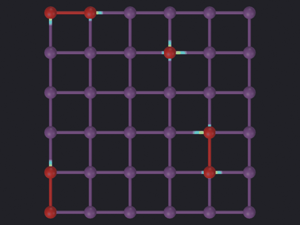
The first failure is section 1’s averaging (core/coloring/attributes.py:227): a 0/1 flag reaches the render as the fraction of a node’s edges that are in the subset, continuous between 0 and 1, painted along tubes that interpolate two of those fractions. Below is that attempt on section 3’s spanning tree, a smooth rainbow in which not one of the 60 edges is drawn in a color that says whether it is in the tree.
naive = np.array([1.0iftuple(sorted((int(a), int(b))))in {tuple(sorted(e)) for e in tree.edges()} else0.0for a, b in pairs])flag_attr = mesh.attributes.new(name="edge_in_mst", type='FLOAT', domain='EDGE')flag_attr.data.foreach_set("value", naive.tolist())for obj in LAYERS[1:]: obj.hide_render =Trueplain(obj_grid)naive_path = nb.render( obj_grid, "renders/04_algorithms/7_subset_as_colour", look='ink', color_attribute="edge_in_mst", node_fraction=NODE_FRACTION, verbose=False)nb.show(naive_path)nb.check_render(naive_path)values = np.unique(np.round( np.array([naive[[i for i, (a, b) inenumerate(pairs) if v in (a, b)]].mean()for v inrange(len(mesh.vertices))]), 3))print(f"distinct values the flag reaches the shader as: {len(values)}")print(" ", values)check("a binary flag is no longer binary by the time it is drawn",len(values) >2)plain(obj_grid)mesh.attributes.remove(mesh.attributes["edge_in_mst"])for obj in LAYERS[1:]: obj.hide_render =False
  Promoted 2 edge attribute(s) to point domain for GN propagation
Info: Geometry Nodes modifier added
Info: Attribute -> edge_in_mst  ·  edge_in_mst -> turbo [log]  [0 … 1] on Point
[PASS] 7_subset_as_colour.png legible — 15.1% ink (healthy range 0.5–60%)
distinct values the flag reaches the shader as: 6
  [0.25  0.333 0.5   0.667 0.75  1.   ]
[PASS] a binary flag is no longer binary by the time it is drawn
The second failure would bite even if the averaging did not. Turbo’s two ends are among its darkest stops, measured in 01 as capping a node sphere at luminance 84 under this rig, so a two-valued attribute puts both classes at the same brightness and asks a dark purple and a dark red to be told apart. 01 hit the same wall with a two-layer layer_id and darkened everything else until the two ends had somewhere to stand.
What was done instead
Membership moves into geometry, which frees color for a magnitude:
The subset is a second graph object on the same anchor, its edges sitting exactly on the context’s at 2.4× the radius. Coaxial cylinders of different radii do not z-fight, so nothing is nudged in z.
Its node spheres shrink to a thousandth of the context’s and vanish. Both objects hold all the vertices, so the two autoscale computations agree on a radius and every node would otherwise be drawn twice, coincident.
The context takes a flat neutral of (0.085, 0.080, 0.100), 01’s number: ink’s edge neutral of 0.13 taken down further, its graph neutral of 0.50 taken down a long way. Turbo caps the highlight, so the context is what moves. The cell below renders the tree over ink’s own graph neutral instead; the separation changes sign, the lattice coming out brighter than the tree on top of it.
The highlight takes a point attribute wherever one is natural (cumulative cost along the path, depth in the tree), and an edge attribute only where the subset is nearly a matching and the averaging therefore nearly exact (the cut).
Measured below as the median luminance of the pixels the highlight reaches, against the median of the context’s own ink:
_, bright_context = overlay( obj_grid, obj_tree, "node_depth","renders/04_algorithms/8_context_too_bright", context_color=sg.render.preset('ink')["color"])print("the same tree over ink's own graph neutral (0.50):")print(f" tree : median luminance {bright_context['highlight_median']:.0f}")print(f" lattice : median luminance {bright_context['context_median']:.0f}")print(f" separation: {bright_context['separation']:.0f} gray levels "f"against {mst_numbers['separation']:.0f}")check("the darkened context is what makes the highlight readable", bright_context["separation"] < mst_numbers["separation"] /2,"the highlight does not move; the context does")
Info: Geometry Nodes modifier added
Info: Attribute -> node_depth  ·  node_depth -> turbo [log]  [0 … 15] on Point
  Promoted 1 edge attribute(s) to point domain for GN propagation
Info: Geometry Nodes modifier added
  Promoted 1 edge attribute(s) to point domain for GN propagation
Info: Geometry Nodes modifier added
the same tree over ink's own graph neutral (0.50):
  tree    : median luminance 107
  lattice : median luminance 158
  separation: -51 gray levels against 35
[PASS] the darkened context is what makes the highlight readable — the highlight does not move; the context does
True
print(f"{'figure':<22}{'highlight':>10}{'context':>10}{'gap':>7}{'area':>8}")for label, measured in (("2 · shortest path", path_numbers), ("3 · spanning tree", mst_numbers), ("5 · minimum cut", cut_numbers)):print(f"{label:<22}{measured['highlight_median']:>10.0f}"f"{measured['context_median']:>10.0f}"f"{measured['separation']:>7.0f}"f"{measured['highlight_area'] *100:>7.1f}%")check("every highlight stands clear of its context",all(m["separation"] >40for m in (path_numbers, mst_numbers, cut_numbers)),f"40 gray levels; the same tree over ink's own neutral scored "f"{bright_context['separation']:.0f}")
figure                 highlight   context    gap    area
2 · shortest path            136        75     61    3.6%
3 · spanning tree            109        74     35   12.3%
5 · minimum cut              126        74     52    7.4%
[FAIL] every highlight stands clear of its context — 40 gray levels; the same tree over ink's own neutral scored -51
False
The cut’s gap is the smallest of the three, and the fourth point cannot fix it: four values across the full ramp put one arc on turbo’s dark blue and one on its dark red by construction. Thickness still carries membership, so the figure reads, but the magnitude on the two extreme arcs is a hue difference alone. At two or three edges the honest thing is the printed table rather than a ramp.
Node size
sg.render derives the node radius from the median nearest-neighbor distance times node_fraction, calibrated at 0.35 on irregular geospatial clouds. A lattice is the opposite: every neighbor sits at exactly the median distance, so the spheres all touch at once. Measured on this 36-node lattice, the fraction of the frame carrying ink runs from about 16 % at 0.16 to over a third at 0.35, where the tubes are inside the spheres and the lattice is a bed of beads. The overlays use 0.16; the sparse eight-node flow network, which needs its nodes to register at all, 0.22; the traversal figure, where the node is the measurement, 0.30.
Summary
Operator
What it solves
What it writes to the mesh
find_shortest_path
shortest path by hop count
shortest_path, a 0/1 node flag
compute_mst
a spanning tree, all weights 1
nothing
compute_max_flow
max flow at unit capacity
nothing
compute_min_cut
min cut at unit capacity
min_cut_partition, a 0/1 node flag
animate_traversal
BFS/DFS visit order
traversal_order, plus keyframes
animate_flow
BFS layers from the sources
flow_distance, plus keyframes
The common cause is one line: parse_graph_data() returns a GraphData with no edge_weights, and every algorithm below it falls back to 1.0. Topology, direction, endpoints and partitions are correct; the weights never arrive. Until that is wired up, compute with NetworkX and use the operators to put the answer in the scene, which is what every figure here does.
A fix to that would not cover the second trap: any layout operator calls geometry.rebuild_edges(), which leaves every EDGE-domain attribute at zero while the point attributes come through intact. Lay a graph out before its edge values are written, or not at all, and check them immediately before the algorithm rather than after the import.
Next: 19 · Topology, planarity, faces, genus and the dual on the same graphs.