05 · Topology

Planarity, faces, genus, duals and crossings, tested against graphs whose answers have been known for a century, because this is the notebook where a wrong result is hardest to notice.

Planarity is right 13 times out of 13, including on two different drawings of the same graph, so the operator reads the graph and not the picture. Euler’s identity holds on every connected planar case, with the outer face counted, and the crossing counts match an independent combinatorial oracle.

What sits on top of that does not hold. The genus routine returns 0 for K₃,₃ and for the Petersen graph, both established as non-planar by the same function moments earlier, because its bound ignores the planarity result it has just computed. Every non-planar graph is reported as containing an “unknown subdivision”, since the call that would identify it goes to a NetworkX function that does not exist.

05 · Topology: planarity, faces, genus, duals and crossings

Every claim below is checked against a value that can be looked up or derived by hand: K₅ and K₃,₃ are not planar, a tree has exactly one face, a connected plane graph satisfies V − E + F = 2, a convex drawing of Kₙ has exactly C(n,4) crossings. Where the add-on disagrees with the mathematics, the disagreement is written down.

The operators are check_planarity, calculate_genus, compute_faces, validate_crossings, visualize_surface, create_dual_graph, toggle_dual_graph, remove_dual_graph, toggle_topo_surface and remove_topo_surface, in SciGraphs/ui/operators/scigraphs/topology_operators.py over SciGraphs/core/algorithms/topology.py, which wraps NetworkX’s Boyer-Myrvold planarity test.

No internet and no data files: every graph is generated.

0 · Setup

import itertools
import math
import pathlib
import random
import sys


def find_repo():
    """Locate the SciGraphs repository, without relying on the cwd.

    In a normal Jupyter the kernel starts per notebook with the cwd set to its
    folder. Not here: the kernel lives inside Blender and existed before you
    opened anything, so the cwd is wherever Blender was launched from. What the
    extension does know is which folder it is serving to JupyterLab.
    """
    candidates = []
    try:
        import bpy
        prefs = bpy.context.preferences.addons[
            "bl_ext.user_default.jupyter_blender"].preferences
        candidates.append(pathlib.Path(bpy.path.abspath(prefs.notebook_dir)))
    except Exception:
        pass
    candidates.append(pathlib.Path.cwd())

    for base in candidates:
        for directory in (base, *base.parents):
            if (directory / "SciGraphs" / "api" / "graphs.py").is_file():
                return directory

    raise RuntimeError(
        "Cannot find the SciGraphs repository. Point at it by hand:\n"
        "    sys.path.insert(0, '/path/to/SciGraphs-1/notebooks/tools')")


sys.path.insert(0, str(find_repo() / "notebooks" / "tools"))

import bpy
import networkx as nx
import numpy as np

# `nb` must import first: it puts this repository on sys.path, so the
# `SciGraphs` import below reads this tree, not the copy Blender installed.
import nb
from nb import check

from SciGraphs import api as sg

# `use_worktree()` puts this repository ahead of the installed add-on for
# `SciGraphs.core.*`, so the cells below can call the same functions the
# operators call. The operators themselves still come from the installed copy.
from scigraphs_core.algorithms import topology
from scigraphs_core.algorithms.graph import GraphData
from scigraphs_core.coloring.colormaps import sample_colormap
from SciGraphs.core.mesh import geometry

SEED = 19
COLLECTION = "SciGraphs_Topology"

print("networkx", nx.__version__)

networkx 3.6

1 · The cast

Eleven graphs in thirteen drawings; two appear twice, drawn two ways, which is what section 6 is for. All are generated from a formula.

sg.graphs.from_gdf() takes GeoDataFrames and none of these graphs is anywhere, so the constructor is SciGraphs.core.mesh.geometry.create_graph_object(), the add-on’s CSV import path. It honors node_coordinates, so the drawing is ours.

Two things that bite. create_graph_object links into bpy.context.collection (SciGraphs/core/mesh/geometry.py:376), which is None under blender -b once the start-up collection has been removed: an AttributeError on a call that has nothing to do with collections. use_collection() below makes one and marks it active first. create_dual_graph does the same at SciGraphs/ui/operators/scigraphs/topology_operators.py:477.

The coordinates are also renormalized to about ten units across. The transform is uniform, so it preserves planarity and every crossing, which is all this notebook reads off the geometry.

Three more properties of that constructor. Node identifiers are stored as one comma-joined string (geometry.py:383 nodes, :394 edges) and split again by layouts/common.py:118 and :126, so a comma inside a label shifts every identifier after it; every label here is str(int). Isolated vertices survive only because the node list is explicit, where the CSV route derives its nodes from the edge list and cannot express a vertex with no edges, which the edgeless cases in section 3 need. And positions are set once, at construction: no layout operator is called, for the reason section 6 gives.

def use_collection(name=COLLECTION):
    """Make `name` the active collection, creating it if necessary."""
    coll = sg.graphs.collection(name)
    view_layer = bpy.context.view_layer
    for layer in view_layer.layer_collection.children:
        if layer.collection is coll:
            view_layer.active_layer_collection = layer
            return coll
    view_layer.active_layer_collection = view_layer.layer_collection
    return coll


def build(graph, positions, name):
    """Materialize a NetworkX graph in Blender at the given 2D positions."""
    use_collection()
    data = GraphData([str(v) for v in graph.nodes()],
                     [(str(u), str(v)) for u, v in graph.edges()])
    data.node_coordinates = {
        str(v): (float(positions[v][0]), float(positions[v][1]), 0.0)
        for v in graph.nodes()}
    with nb.quiet():
        obj = geometry.create_graph_object(data, is_directed=False,
                                           remove_self_loops=True)
    obj.name = name
    obj.data.name = f"{name}_Mesh"
    obj["topo_case"] = name
    return obj


def act(obj):
    """Make `obj` the active and only selected object, headless-safe."""
    for other in bpy.data.objects:
        other.select_set(False)
    bpy.context.view_layer.objects.active = obj
    obj.select_set(True)
    return obj


def convex(graph, radius=5.0):
    """The convex (circular) drawing: every node on a circle, in node order."""
    count = graph.number_of_nodes()
    return {v: (radius * math.cos(2 * math.pi * i / count),
            radius * math.sin(2 * math.pi * i / count))
            for i, v in enumerate(graph.nodes())}

The one graph that is not a textbook name: a 6 × 6 lattice with twelve edges knocked out. A plain grid has faces of one size; perforating it spreads the sizes while keeping the answer computable. The removals are seeded, and each is kept only if the result stays connected with no node of degree 1, since a degree-1 node adds a dangling edge and those are section 5’s topic.

def perforated_grid(side=6, cuts=12, seed=SEED):
    base = nx.grid_2d_graph(side, side)
    order = list(base.nodes())
    rng = random.Random(seed)
    candidates = sorted(base.edges())
    rng.shuffle(candidates)
    removed = 0
    for u, v in candidates:
        if removed >= cuts:
            break
        base.remove_edge(u, v)
        if nx.is_connected(base) and min(d for _, d in base.degree()) >= 2:
            removed += 1
        else:
            base.add_edge(u, v)
    mapping = {v: i for i, v in enumerate(order)}
    graph = nx.relabel_nodes(base, mapping)
    positions = {mapping[v]: (float(v[0]), float(v[1])) for v in order}
    return graph, positions, removed


grid, grid_pos, cuts_made = perforated_grid()

lattice = nx.triangular_lattice_graph(5, 9)
lattice_pos = nx.get_node_attributes(lattice, "pos")
lattice = nx.convert_node_labels_to_integers(lattice, label_attribute="orig")
lattice_pos = {i: lattice.nodes[i]["pos"] for i in lattice.nodes()}

tree = nx.balanced_tree(2, 3)
octahedron = nx.octahedral_graph()
two_triangles = nx.disjoint_union(nx.cycle_graph(3), nx.cycle_graph(3))
two_triangles_pos = {0: (-3, 0), 1: (-1, 0), 2: (-2, 2),
                     3: (1, 0), 4: (3, 0), 5: (2, 2)}

# The last column is from the literature, not from NetworkX: checking
# `check_planarity_nx` against `nx.check_planarity` would only prove that a
# wrapper wraps.
CAST = [
    # name             graph                              drawing            planar
    ("Grid",           grid,                              grid_pos,          True),
    ("Lattice",        lattice,                           lattice_pos,       True),
    ("Tree",           tree,                              None,              True),
    ("C4",             nx.cycle_graph(4),                 None,              True),
    ("Octahedron",     octahedron,                        None,              True),
    ("Octa_convex",    octahedron,                        convex(octahedron), True),
    ("Grid_convex",    grid,                              convex(grid, 6.0), True),
    ("TwoTriangles",   two_triangles,                     two_triangles_pos, True),
    ("K5",             nx.complete_graph(5),              None,              False),
    ("K33",            nx.complete_bipartite_graph(3, 3), None,              False),
    ("K7",             nx.complete_graph(7),              None,              False),
    ("K8",             nx.complete_graph(8),              None,              False),
    ("Petersen",       nx.petersen_graph(),               None,              False),
]

sg.graphs.clear_scene(keep_anchor=False)

objects, graphs, known_planar = {}, {}, {}
for name, graph, positions, planar in CAST:
    if positions is None:
        positions = (nx.planar_layout(graph, scale=5.0) if planar
                     else convex(graph))
    objects[name] = build(graph, positions, name)
    graphs[name] = graph
    known_planar[name] = planar

print(f"perforated grid: {cuts_made} edges removed, "
      f"connected={nx.is_connected(grid)}")
print(f"{len(objects)} graphs in the scene\n")
print(f"{'name':<14}{'V':>4}{'E':>5}   known")
for name, graph, _positions, planar in CAST:
    print(f"{name:<14}{graph.number_of_nodes():>4}{graph.number_of_edges():>5}"
          f"   {'planar' if planar else 'NOT planar'}")

check("every graph reached the scene",
      all(obj is not None for obj in objects.values()))
check("the drawings survived the renormalization",
      all(len(obj.data.vertices) == graphs[name].number_of_nodes()
      for name, obj in objects.items()))


Creating graph object with 36 nodes...
  Coordinates applied for 36/36 nodes in 0.00s
  Vertices created in 0.00s
  48 edges created in 0.00s
  Mesh conversion in 0.00s
  Object created in 0.00s
Total graph creation time: 0.00s

Creating graph object with 33 nodes...
  Coordinates applied for 33/33 nodes in 0.00s
  Vertices created in 0.00s
  77 edges created in 0.00s
  Mesh conversion in 0.00s
  Object created in 0.00s
Total graph creation time: 0.00s

Creating graph object with 15 nodes...
  Coordinates applied for 15/15 nodes in 0.00s
  Vertices created in 0.00s
  14 edges created in 0.00s
  Mesh conversion in 0.00s
  Object created in 0.00s
Total graph creation time: 0.00s

Creating graph object with 4 nodes...
  Coordinates applied for 4/4 nodes in 0.00s
  Vertices created in 0.00s
  4 edges created in 0.00s
  Mesh conversion in 0.00s
  Object created in 0.00s
Total graph creation time: 0.00s

Creating graph object with 6 nodes...
  Coordinates applied for 6/6 nodes in 0.00s
  Vertices created in 0.00s
  12 edges created in 0.00s
  Mesh conversion in 0.00s
  Object created in 0.00s
Total graph creation time: 0.00s

Creating graph object with 6 nodes...
  Coordinates applied for 6/6 nodes in 0.00s
  Vertices created in 0.00s
  12 edges created in 0.00s
  Mesh conversion in 0.00s
  Object created in 0.00s
Total graph creation time: 0.00s

Creating graph object with 36 nodes...
  Coordinates applied for 36/36 nodes in 0.00s
  Vertices created in 0.00s
  48 edges created in 0.00s
  Mesh conversion in 0.00s
  Object created in 0.00s
Total graph creation time: 0.00s

Creating graph object with 6 nodes...
  Coordinates applied for 6/6 nodes in 0.00s
  Vertices created in 0.00s
  6 edges created in 0.00s
  Mesh conversion in 0.00s
  Object created in 0.00s
Total graph creation time: 0.00s

Creating graph object with 5 nodes...
  Coordinates applied for 5/5 nodes in 0.00s
  Vertices created in 0.00s
  10 edges created in 0.00s
  Mesh conversion in 0.00s
  Object created in 0.00s
Total graph creation time: 0.00s

Creating graph object with 6 nodes...
  Coordinates applied for 6/6 nodes in 0.00s
  Vertices created in 0.00s
  9 edges created in 0.00s
  Mesh conversion in 0.00s
  Object created in 0.00s
Total graph creation time: 0.00s

Creating graph object with 7 nodes...
  Coordinates applied for 7/7 nodes in 0.00s
  Vertices created in 0.00s
  21 edges created in 0.00s
  Mesh conversion in 0.00s
  Object created in 0.00s
Total graph creation time: 0.00s

Creating graph object with 8 nodes...
  Coordinates applied for 8/8 nodes in 0.00s
  Vertices created in 0.00s
  28 edges created in 0.00s
  Mesh conversion in 0.00s
  Object created in 0.00s
Total graph creation time: 0.00s

Creating graph object with 10 nodes...
  Coordinates applied for 10/10 nodes in 0.00s
  Vertices created in 0.00s
  15 edges created in 0.00s
  Mesh conversion in 0.00s
  Object created in 0.00s
Total graph creation time: 0.00s
perforated grid: 12 edges removed, connected=True
13 graphs in the scene

name             V    E   known
Grid            36   48   planar
Lattice         33   77   planar
Tree            15   14   planar
C4               4    4   planar
Octahedron       6   12   planar
Octa_convex      6   12   planar
Grid_convex     36   48   planar
TwoTriangles     6    6   planar
K5               5   10   NOT planar
K33              6    9   NOT planar
K7               7   21   NOT planar
K8               8   28   NOT planar
Petersen        10   15   NOT planar
[PASS] every graph reached the scene
[PASS] the drawings survived the renormalization

True

2 · Planarity

check_planarity runs NetworkX’s Boyer-Myrvold test and stores topo_is_planar on the object, plus the Euler quadruple when the graph is planar. Kuratowski’s theorem is why the two non-planar cases below are the canonical ones: a graph is planar iff it contains no subdivision of K₅ or K₃,₃, the two smallest obstructions (K₅ by vertices, K₃,₃ by edges).

verdicts = {}
for name in objects:
    act(objects[name])
    with nb.quiet():
        bpy.ops.scigraphs.check_planarity()
    verdicts[name] = bool(objects[name]["topo_is_planar"])

wrong = [n for n in verdicts if verdicts[n] != known_planar[n]]
for name in objects:
    mark = "ok " if verdicts[name] == known_planar[name] else "WRONG"
    print(f"  {name:<14} operator says {'planar' if verdicts[name] else 'NOT planar':<10}"
          f" known {'planar' if known_planar[name] else 'NOT planar':<10} {mark}")

check("the planarity test agrees with the literature on all 13 graphs",
      not wrong, f"disagreements: {wrong}" if wrong else "")

Info: Graph is PLANAR: V=36, E=48, F=14, chi=2
Info: Graph is PLANAR: V=33, E=77, F=46, chi=2
Info: Graph is PLANAR: V=15, E=14, F=1, chi=2
Info: Graph is PLANAR: V=4, E=4, F=2, chi=2
Info: Graph is PLANAR: V=6, E=12, F=8, chi=2
Info: Graph is PLANAR: V=6, E=12, F=8, chi=2
Info: Graph is PLANAR: V=36, E=48, F=14, chi=2
Info: Graph is PLANAR: V=6, E=6, F=4, chi=4
Warning: Graph is NON-PLANAR (contains unknown subdivision)
Warning: Graph is NON-PLANAR (contains unknown subdivision)
Warning: Graph is NON-PLANAR (contains unknown subdivision)
Warning: Graph is NON-PLANAR (contains unknown subdivision)
Warning: Graph is NON-PLANAR (contains unknown subdivision)
  Grid           operator says planar     known planar     ok 
  Lattice        operator says planar     known planar     ok 
  Tree           operator says planar     known planar     ok 
  C4             operator says planar     known planar     ok 
  Octahedron     operator says planar     known planar     ok 
  Octa_convex    operator says planar     known planar     ok 
  Grid_convex    operator says planar     known planar     ok 
  TwoTriangles   operator says planar     known planar     ok 
  K5             operator says NOT planar known NOT planar ok 
  K33            operator says NOT planar known NOT planar ok 
  K7             operator says NOT planar known NOT planar ok 
  K8             operator says NOT planar known NOT planar ok 
  Petersen       operator says NOT planar known NOT planar ok 
[PASS] the planarity test agrees with the literature on all 13 graphs

True

Both drawings of the octahedron come back planar, and so does the circular drawing of the grid: planarity is a property of the graph, and check_planarity never looks at the vertex positions. Section 6 is about the operator that does.

When the answer is no, the branch that reports it tries to name the obstruction it found, and cannot.

act(objects["K5"])
print("K5 stored kuratowski type:", objects["K5"].get("topo_kuratowski_type"))
print("K33 stored kuratowski type:", objects["K33"].get("topo_kuratowski_type"))

probe = topology.detect_kuratowski_subgraph(
    GraphData([str(v) for v in nx.complete_graph(5).nodes()],
              [(str(u), str(v)) for u, v in nx.complete_graph(5).edges()]))
print("detect_kuratowski_subgraph ->", probe)
print("networkx has planarity.kuratowski_subgraph:",
      hasattr(nx.algorithms.planarity, "kuratowski_subgraph"))

K5 stored kuratowski type: unknown
K33 stored kuratowski type: unknown
detect_kuratowski_subgraph -> {'is_planar': False, 'kuratowski_type': 'unknown', 'subgraph_nodes': None}
networkx has planarity.kuratowski_subgraph: False

Operator defect. topology.detect_kuratowski_subgraph calls nx.algorithms.planarity.kuratowski_subgraph(G) (SciGraphs/core/algorithms/topology.py:356). No such function exists in NetworkX, in 3.6 or any release. The call raises AttributeError, the bare except Exception two lines below (topology.py:374) swallows it, and the function returns kuratowski_type='unknown' for every non-planar graph. The operator reports “Graph is NON-PLANAR (contains unknown subdivision)” (topology_operators.py:52), which reads like a hedge and is dead code.

nx.check_planarity(G, counterexample=True) returns a Kuratowski subgraph as its second element. The classification below it (K₅ if the subgraph has ≥ 5 nodes and ≥ 10 edges, K₃,₃ otherwise, topology.py:364) is also wrong on its own terms: a subdivision of K₃,₃ with two extra vertices has 11 edges and would be reported as K₅.

3 · Faces and Euler’s formula

compute_faces traverses the rotation system of the planar embedding and writes topo_num_faces on the object and a face_id integer attribute on the mesh. The number on its own is not checkable; the identity is:

For a connected graph drawn in the plane, V − E + F = 2, counting the unbounded outer face.

So the test is not “does it return 14” but “does 36 − 48 + 14 equal 2”.

connected_planar = ["Grid", "Lattice", "Tree", "C4", "Octahedron"]

print(f"{'name':<12}{'V':>4}{'E':>5}{'F':>5}{'chi':>6}   V-E+F")
euler_ok = True
for name in connected_planar:
    obj = objects[name]
    act(obj)
    with nb.quiet():
        bpy.ops.scigraphs.compute_faces()
    V = int(obj["topo_euler_V"])
    E = int(obj["topo_euler_E"])
    F = int(obj["topo_num_faces"])
    chi = V - E + F
    euler_ok = euler_ok and chi == 2
    print(f"{name:<12}{V:>4}{E:>5}{F:>5}{chi:>6}   {V} - {E} + {F} = {chi}")

check("V - E + F = 2 on every connected planar graph in the cast",
      euler_ok)

name           V    E    F   chi   V-E+F
Info: Found 14 faces. Attribute 'face_id' created.
Grid          36   48   14     2   36 - 48 + 14 = 2
Info: Found 46 faces. Attribute 'face_id' created.
Lattice       33   77   46     2   33 - 77 + 46 = 2
Info: Found 1 faces. Attribute 'face_id' created.
Tree          15   14    1     2   15 - 14 + 1 = 2
Info: Found 2 faces. Attribute 'face_id' created.
C4             4    4    2     2   4 - 4 + 2 = 2
Info: Found 8 faces. Attribute 'face_id' created.
Octahedron     6   12    8     2   6 - 12 + 8 = 2
[PASS] V - E + F = 2 on every connected planar graph in the cast

True

The tree decides whether the outer face is counted. A tree has no cycle, so it bounds no region: the only face is the unbounded one and F must be 1. An implementation that dropped the outer face would return 0 here, and V − E + F would come out 1 instead of 2.

V, E = tree.number_of_nodes(), tree.number_of_edges()
F = int(objects["Tree"]["topo_num_faces"])
print(f"tree: V={V} E={E} F={F}  (E = V - 1 = {V - 1}, so F must be 1)")
check("the outer face is counted", F == 1)

tree: V=15 E=14 F=1  (E = V - 1 = 14, so F must be 1)
[PASS] the outer face is counted

True

Every edge lies on exactly two face boundaries (the same face twice if it is a bridge), so

Σ deg(f) = 2E

which catches a traversal that walks an edge once instead of twice. topo_faces is the face list itself, stored as the repr() of a list of lists of node indices.

faces_grid = eval(objects["Grid"]["topo_faces"])
degrees = sorted(len(face) for face in faces_grid)
print("grid face degrees:", degrees)
print(f"sum {sum(degrees)}   2E = {2 * grid.number_of_edges()}")
check("every edge is on exactly two face boundaries",
      sum(degrees) == 2 * grid.number_of_edges())

grid face degrees: [4, 4, 4, 4, 4, 4, 4, 4, 6, 6, 8, 12, 12, 20]
sum 96   2E = 96
[PASS] every edge is on exactly two face boundaries

True

Where the identity stops holding

Two boundary cases, both accepted without complaint.

Disconnected graphs. TwoTriangles is two disjoint triangles. Drawn in the plane they share one unbounded face, so the honest count is F = 3 and the generalized identity is V − E + F = 1 + C, with C the number of components: 6 − 6 + 3 = 3.

act(objects["TwoTriangles"])
with nb.quiet():
    bpy.ops.scigraphs.check_planarity()
obj = objects["TwoTriangles"]
V = int(obj["topo_euler_V"])
E = int(obj["topo_euler_E"])
F = int(obj["topo_euler_F"])
components = nx.number_connected_components(two_triangles)
print(f"V={V} E={E} F={F} chi={obj['topo_euler_chi']}  components={components}")
print(f"  drawn in one plane:      V - E + F = 1 + C = {1 + components}, so F = {E - V + 1 + components}")
print(f"  one sphere per component: V - E + F = 2C = {2 * components}, so F = {E - V + 2 * components}")

check("the reported chi is 2C, not 2",
      V - E + F == 2 * components,
      f"{V} - {E} + {F} = {V - E + F}")

Info: Graph is PLANAR: V=6, E=6, F=4, chi=4
V=6 E=6 F=4 chi=4  components=2
  drawn in one plane:      V - E + F = 1 + C = 3, so F = 3
  one sphere per component: V - E + F = 2C = 4, so F = 4
[PASS] the reported chi is 2C, not 2 — 6 - 6 + 4 = 4

True

Worth knowing rather than a defect. The face traversal walks each component’s outer boundary separately (topology.py:125), so it counts one outer face per component. That is the Euler characteristic of C disjoint spheres, χ = 2C, and the only answer available from a combinatorial embedding, which does not record how the components are nested in a common plane. The docstring above it says otherwise, “For planar graphs embedded in a plane: chi = 2” (topology.py:62), and the operator reports chi=4 for a graph it calls planar. Read topo_euler_chi as 2C and check connectivity yourself before believing a 2.

Graphs with no edges. An isolated vertex has no half-edges, so the traversal never starts and it contributes no face at all, not even the one it sits in.

for label, graph in (("one isolated node", nx.empty_graph(1)),
                     ("three isolated nodes", nx.empty_graph(3)),
                     ("triangle + isolated node",
                     nx.disjoint_union(nx.cycle_graph(3), nx.empty_graph(1)))):
    data = GraphData([str(v) for v in graph.nodes()],
                     [(str(u), str(v)) for u, v in graph.edges()])
    planar, embedding = topology.check_planarity_nx(data)
    euler = topology.get_euler_characteristic(data, embedding)
    parts = nx.number_connected_components(graph)
    print(f"  {label:<26} V={euler['V']} E={euler['E']} "
          f"F={euler['F']} chi={euler['chi']}   expected chi=2C={2 * parts}")

check("an edgeless component contributes no face at all",
      topology.get_euler_characteristic(
      GraphData(["0"], []),
      topology.check_planarity_nx(GraphData(["0"], []))[1])["F"] == 0,
      "F=0 for a single node; a point drawn in the plane has one face")

  one isolated node          V=1 E=0 F=0 chi=1   expected chi=2C=2
  three isolated nodes       V=3 E=0 F=0 chi=3   expected chi=2C=6
  triangle + isolated node   V=4 E=3 F=2 chi=3   expected chi=2C=4
[PASS] an edgeless component contributes no face at all — F=0 for a single node; a point drawn in the plane has one face

True

`face_id`, and what it is not

compute_faces also writes a point attribute, which reads as “which face this node belongs to” and is not that: a node belongs to as many faces as it has incident edges. It holds the lowest-numbered face containing the node (topology.py:414), an artifact of the traversal order.

obj = objects["Grid"]
attr = obj.data.attributes["face_id"]
values = np.array([attr.data[i].value for i in range(len(obj.data.vertices))])
used = sorted(set(values.tolist()))
print(f"faces found          {obj['topo_num_faces']}")
print(f"distinct face_id     {len(used)}  ->  {used}")
print(f"nodes on face 0      {int((values == used[0]).sum())} of {len(values)}")

check("face_id is not a partition of the faces",
      len(used) < int(obj["topo_num_faces"]),
      f"{len(used)} labels for {obj['topo_num_faces']} faces")

faces found          14
distinct face_id     6  ->  [0, 1, 2, 3, 6, 11]
nodes on face 0      6 of 36
[PASS] face_id is not a partition of the faces — 6 labels for 14 faces

True

The suite’s style: look='ink' and its turbo ramp, straight down through an orthographic camera (render_eevee’s default). The color is face_id, on the POINT domain, so it lands on the node spheres and the tubes take a neutral.

A face label is categorical and turbo is a continuous ramp. Notebook 06 measures this on 18 K-Means labels and finds the closest adjacent pair 55/765 apart in turbo, the best of the five colormaps in the set and still not a categorical scale. Six labels is easier, and the separations are measured below rather than assumed.

Notebook 13 diagnosed the other half. Turbo’s two endpoints are its darkest stops, so the lowest and highest labels get the dimmest colors available, and ink’s default edge_color of 0.13 renders tubes brighter than they are, putting the measurement underneath the wiring. 01 pushed the neutral below both ends and its value is not low enough. Median luminance out of 255, projecting every node center through the camera and reading the render back:

`edge_color`	tubes (median / p90)	darkest label
0.130, ink’s default	98 / 102	84	tubes 14 levels over the data
0.085, notebook 13’s	85 / 89	81	still over
0.060	75 / 80	83	under both endpoints
0.045	69 / 75	80	under, and the wiring starts to vanish

The two dark classes are the two ends: label 0 at 88 and label 11 at 83, against 148, 175, 185 and 221 for the four in between. The difference from 01 is the tube radius: these lattices have a wide node spacing, so edge_ratio puts more lit surface on every tube.

ramp = sample_colormap("turbo", samples=256)
low, high = min(used), max(used)


def turbo_at(value):
    position = 0.0 if high == low else (value - low) / (high - low)
    return np.asarray(ramp[int(round(position * 255))][:3], dtype=float) * 255.0


separations = [float(np.abs(turbo_at(used[i + 1]) - turbo_at(used[i])).sum())
               for i in range(len(used) - 1)]
print("turbo separation between adjacent labels, out of 765:",
      [round(s) for s in separations])
print(f"closest pair: {round(min(separations))}/765 "
      f"(notebook 18 measures 55/765 at 18 labels)")

check("no two adjacent labels are closer than 06's 18-label worst case",
      min(separations) >= 55,
      f"{round(min(separations))}/765")

turbo separation between adjacent labels, out of 765: [220, 118, 128, 372, 358]
closest pair: 118/765 (notebook 18 measures 55/765 at 18 labels)
[PASS] no two adjacent labels are closer than 06's 18-label worst case — 118/765

True

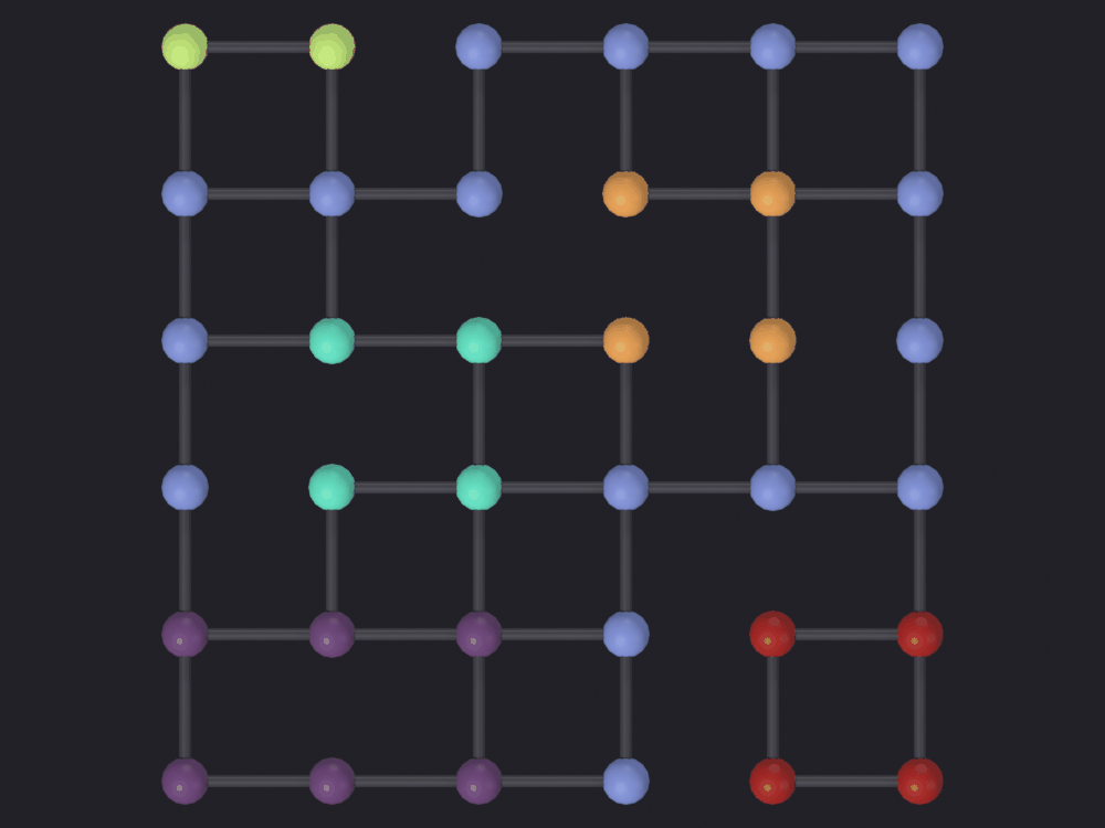
node_fraction=0.16, well below the 0.35 default. That default is calibrated on an irregular point cloud with room between the clusters; a lattice is the case the README’s “string of beads” warning is about. Measured on this figure: 0.35 gives 34 % ink with the grid buried under its own nodes, 0.22 gives 20 %, and 0.16 gives 13 % with every cut edge visible as a gap. A figure about faces has to show those, since the faces are exactly the gaps.

LABEL_EDGE_COLOR = (0.060, 0.056, 0.071)   # measured above; 01's hue, lower value

nb.figure(objects["Grid"], "renders/17_topology/1_faces",
          look='ink', color_attribute="face_id",
          node_fraction=0.16, edge_color=LABEL_EDGE_COLOR)

Info: Geometry Nodes modifier added
Info: Attribute -> face_id  ·  face_id -> turbo [log]  [0 … 11] on Point

[PASS] 1_faces.png legible — 13.4% ink (healthy range 0.5–60%)

The label steps up as the traversal works across the drawing, and the nodes sharing a color are the ones it reached first from the same face. Read as “the faces of this graph”, which the name invites, it is wrong: 14 faces, 6 colors. The dual, next, is the figure that does show the faces.

4 · Genus

The genus of a graph is the smallest number of handles a surface needs before the graph can be drawn on it without crossings. Planar graphs have genus 0; K₅, K₃,₃, K₇ and the Petersen graph have genus 1, drawing cleanly on a torus; K₈ has genus 2.

Computing it exactly is NP-hard (Thomassen, 1989), so calculate_genus returns two different things instead (SciGraphs/core/algorithms/topology.py:263):

planar → genus_exact = 0, genus_lower_bound = 0. Exact: planarity is decidable in linear time and genus 0 follows.
non-planar → genus_exact = None and genus_lower_bound = ceil((E − 3V + 6) / 6). A lower bound, never an estimate and never an upper bound, from Euler’s inequality for a graph of girth 3 on an orientable surface of genus g: E ≤ 3(V − 2 + 2g).

The report line says Genus >= n for the second case, the correct reading. topo_genus_exact is not written when the graph is not planar; its absence is the signal.

GENUS_KNOWN = {"K5": 1, "K33": 1, "K7": 1, "K8": 2, "Petersen": 1,
               "Grid": 0, "Lattice": 0, "Tree": 0, "C4": 0, "Octahedron": 0}

print(f"{'name':<12}{'V':>4}{'E':>5}{'bound':>7}{'exact':>7}   known genus")
bounds = {}
for name in GENUS_KNOWN:
    obj = objects[name]
    act(obj)
    if "topo_genus_exact" in obj.keys():
        del obj["topo_genus_exact"]
    with nb.quiet():
        bpy.ops.scigraphs.calculate_genus()
    bound = int(obj["topo_genus_lower_bound"])
    exact = obj.get("topo_genus_exact")
    bounds[name] = bound
    flag = "" if bound <= GENUS_KNOWN[name] else "  BOUND ABOVE THE TRUTH"
    print(f"{name:<12}{obj['topo_euler_V']:>4}{obj['topo_euler_E']:>5}"
          f"{bound:>7}{str(exact):>7}   {GENUS_KNOWN[name]}{flag}")

check("the bound is never above the true genus",
      all(bounds[n] <= GENUS_KNOWN[n] for n in GENUS_KNOWN))
check("genus is exact exactly when the graph is planar",
      all((objects[n].get("topo_genus_exact") is not None)
      == known_planar[n] for n in GENUS_KNOWN))

name           V    E  bound  exact   known genus
Info: Genus >= 1 (non-planar): V=5, E=10
K5             5   10      1   None   1
Info: Genus >= 0 (non-planar): V=6, E=9
K33            6    9      0   None   1
Info: Genus >= 1 (non-planar): V=7, E=21
K7             7   21      1   None   1
Info: Genus >= 2 (non-planar): V=8, E=28
K8             8   28      2   None   2
Info: Genus >= 0 (non-planar): V=10, E=15
Petersen      10   15      0   None   1
Info: Genus = 0 (planar): V=36, E=48, F=14
Grid          36   48      0      0   0
Info: Genus = 0 (planar): V=33, E=77, F=46
Lattice       33   77      0      0   0
Info: Genus = 0 (planar): V=15, E=14, F=1
Tree          15   14      0      0   0
Info: Genus = 0 (planar): V=4, E=4, F=2
C4             4    4      0      0   0
Info: Genus = 0 (planar): V=6, E=12, F=8
Octahedron     6   12      0      0   0
[PASS] the bound is never above the true genus
[PASS] genus is exact exactly when the graph is planar

True

The bound is tight on K₅, K₇ and K₈ (1, 1 and 2, the true genera), and for the right reason: those are the graphs whose faces really can all be triangles. On K₃,₃ and the Petersen graph it returns 0, for a graph the same function declared non-planar two lines earlier. A non-planar graph has genus at least 1 by definition, so 0 contradicts the result already in hand.

for name in ("K33", "Petersen"):
    graph = graphs[name]
    V, E = graph.number_of_nodes(), graph.number_of_edges()
    girth = nx.girth(graph)
    triangle_bound = math.ceil((E - 3 * V + 6) / 6)
    # Euler's inequality with the real girth: E <= g/(g-2) * (V - 2 + 2g_enus)
    girth_bound = math.ceil((((girth - 2) * E) / girth - V + 2) / 2)
    print(f"{name:<10} V={V} E={E} girth={girth}  "
          f"girth-3 bound {triangle_bound} -> reported {bounds[name]}   "
          f"girth-aware bound {girth_bound}   true genus {GENUS_KNOWN[name]}")

contradiction = [n for n in ("K5", "K33", "K7", "K8", "Petersen")
                 if bounds[n] < 1]
print(f"\nnon-planar graphs reported with a genus bound of 0: {contradiction}")

check("a girth-aware bound recovers genus >= 1 on both of them",
      all(math.ceil(((((nx.girth(graphs[n]) - 2) * graphs[n].number_of_edges())
      / nx.girth(graphs[n])) - graphs[n].number_of_nodes() + 2) / 2) >= 1
      for n in contradiction))

K33        V=6 E=9 girth=4  girth-3 bound 0 -> reported 0   girth-aware bound 1   true genus 1
Petersen   V=10 E=15 girth=5  girth-3 bound -1 -> reported 0   girth-aware bound 1   true genus 1

non-planar graphs reported with a genus bound of 0: ['K33', 'Petersen']
[PASS] a girth-aware bound recovers genus >= 1 on both of them

True

Operator defect. topology.calculate_genus computes max(0, ceil((E − 3V + 6) / 6)) at SciGraphs/core/algorithms/topology.py:307 and returns it as genus_lower_bound without consulting the planarity result it computed at line 288. The formula assumes every face is a triangle, right for a complete graph and wrong for anything triangle-free: K₃,₃ is bipartite (girth 4) and the Petersen graph has girth 5, so their faces need at least 4 and 5 edges. Either one-line repair fixes both cases: max(1, …) when is_planar is False, or the girth-aware inequality E ≤ g/(g − 2) · (V − 2 + 2g_enus) computed above. The report line reads “Genus >= 0 (non-planar)”, a statement true of every graph in existence, printed as though it were a measurement.

5 · The dual graph

create_dual_graph builds the geometric dual G*: one vertex per face of the planar embedding, placed at that face’s centroid, and an edge between two faces for every edge of G they share. It needs a planar embedding, so it refuses on a non-planar graph and before check_planarity has run.

The checkable claim is the first half: |V(G*)| = F.

act(objects["Grid"])
with nb.quiet():
    bpy.ops.scigraphs.create_dual_graph()
dual = bpy.data.objects[objects["Grid"]["topo_dual_child"]]
# The operator parents the dual to the primal, so it inherits the primal's
# transform in every later render. Nothing here moves the primal, but that is
# a trap for whoever does.
dual.parent = None

faces = eval(objects["Grid"]["topo_faces"])
print(f"primal   V={grid.number_of_nodes()} E={grid.number_of_edges()} F={len(faces)}")
print(f"dual     V*={dual['num_nodes']} E*={dual['num_edges']} "
      f"(mesh: {len(dual.data.vertices)} verts, {len(dual.data.edges)} edges)")

check("the dual has one vertex per face",
      int(dual["num_nodes"]) == len(faces),
      f"{dual['num_nodes']} vs {len(faces)} faces")

Info: Dual graph created: 14 faces -> vertices, 29 shared edges -> dual edges
primal   V=36 E=48 F=14
dual     V*=14 E*=29 (mesh: 14 verts, 28 edges)
[PASS] the dual has one vertex per face — 14 vs 14 faces

True

The second half diverges. A geometric dual has exactly as many edges as the primal, because each primal edge is crossed by exactly one dual edge. This one has fewer, for two separate reasons.

bridges = list(nx.bridges(grid))
parallel = grid.number_of_edges() - int(dual["num_edges"])
print(f"primal edges                {grid.number_of_edges()}")
print(f"dual edges reported         {dual['num_edges']}")
print(f"dual edges in the mesh      {len(dual.data.edges)}")
print(f"bridges in the primal       {len(bridges)}  -> dual self-loops")
print(f"lost to the de-duplication  {parallel}")

check("the dual is missing edges the mathematics requires",
      int(dual["num_edges"]) < grid.number_of_edges(),
      f"{dual['num_edges']} vs {grid.number_of_edges()}")
check("the dual mesh holds fewer edges still than the operator reports",
      len(dual.data.edges) < int(dual["num_edges"]),
      f"{len(dual.data.edges)} in the mesh, {dual['num_edges']} reported")

primal edges                48
dual edges reported         29
dual edges in the mesh      28
bridges in the primal       1  -> dual self-loops
lost to the de-duplication  19
[PASS] the dual is missing edges the mathematics requires — 29 vs 48
[PASS] the dual mesh holds fewer edges still than the operator reports — 28 in the mesh, 29 reported

True

Operator limitation. The dual of a planar graph is in general a multigraph: two faces sharing three edges are joined by three dual edges, and a bridge (an edge with the same face on both sides) becomes a dual self-loop. Neither survives here.

topology.compute_geometric_dual_3d collects the dual edges as unordered pairs and then does dual_edges = list(set(dual_edges)) (SciGraphs/core/algorithms/topology.py:246), collapsing every parallel class to one edge. The bridges do produce their (f, f) pairs, so they are counted in num_edges, but bmesh.edges.new([v, v]) raises and the except ValueError: pass at topology_operators.py:468 drops them, which is why the stored num_edges is above what the mesh holds. Any dual read out of this object is the simple dual, and V* − E* + F* will not come back to 2.

The other dual in this suite

Notebook 17 uses bpy.ops.scigraphs.create_street_dual_graph(). The shared word misleads; the constructions are unrelated:

	`create_dual_graph` (here)	`create_street_dual_graph` (notebook 17)
What a node is	a face of a planar embedding	a street segment
What an edge is	two faces sharing a primal edge	two segments sharing an intersection
Needs planarity	yes, refuses otherwise	no
Needs a drawing	yes, nodes sit at face centroids	no
Node count	F	E of the primal
Mathematically	the geometric dual G*	the line graph L(G)

The line graph exists for every graph; the geometric dual only for a planar one, and it depends on the embedding, so two isomorphic planar graphs can have non-isomorphic duals. Neither is a special case of the other, and nothing in the add-on’s UI says so.

line_nodes = grid.number_of_edges()
line_edges = sum(d * (d - 1) // 2 for _, d in grid.degree())
print(f"grid: V={grid.number_of_nodes()} E={grid.number_of_edges()} F={len(faces)}")
print(f"  geometric dual  V*={dual['num_nodes']:<4} (= F)")
print(f"  line graph      V ={line_nodes:<4} (= E), E = {line_edges}")
check("the two duals do not even have the same number of nodes",
      int(dual["num_nodes"]) != line_nodes)

grid: V=36 E=48 F=14
  geometric dual  V*=14   (= F)
  line graph      V =48   (= E), E = 89
[PASS] the two duals do not even have the same number of nodes

True

The dual carries no attribute of its own, so the figure needs one: the size of the face each dual node stands for, a 4-gon, a 6-gon, the 20-gon that is the outer boundary. It varies, which is why the grid was perforated in section 1.

face_degrees = [len(face) for face in faces]
mesh = dual.data
if "face_degree" in mesh.attributes:
    mesh.attributes.remove(mesh.attributes["face_degree"])
attr = mesh.attributes.new(name="face_degree", type='INT', domain='POINT')
attr.data.foreach_set("value", face_degrees[:len(mesh.vertices)])
print("face degrees:", sorted(face_degrees))

face degrees: [4, 4, 4, 4, 4, 4, 4, 4, 6, 6, 8, 12, 12, 20]

clip_high_pct=98 because the distribution has one member two thirds larger than the next: eight 4-gons, two 6-gons, one 8-gon, two 12-gons, and the outer face bounded by the whole 20-edge perimeter. Left unclipped the outer face takes the top of the ramp on its own and everything below a 12-gon is pressed into the bottom stop, the comparison the figure is for.

vmin/vmax would say the same thing and are silently ineffective: scigraphs.color_set_attribute calls fn.update_property_range() before reading them (SciGraphs/ui/coloring/operators.py:374) and overwrites both. The percentile pair is the one that survives.

nb.figure(dual, "renders/17_topology/2_dual",
          look='ink', color_attribute="face_degree",
          clip_high_pct=98, node_fraction=0.20,
          edge_color=LABEL_EDGE_COLOR)

Info: Geometry Nodes modifier added
Info: Attribute -> face_degree  ·  face_degree -> turbo [log]  [4 … 17.92] on Point

[PASS] 2_dual.png legible — 16.3% ink (healthy range 0.5–60%)

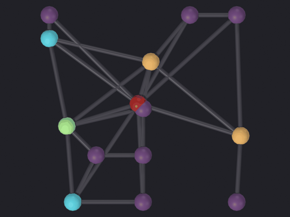
Each sphere is a face of the graph in figure 1, sitting where that face is, colored by how many edges bound it: purple for the 4-gons of the intact lattice, blue, cyan and yellow for the larger faces the twelve cuts opened, red for the outer face.

The red one sits in the middle, half hidden behind a purple one, and no node size fixes it. The outer face is unbounded, so its natural position is outside everything or at infinity, but compute_geometric_dual_3d places every dual vertex at the arithmetic mean of its face’s corners (topology.py:214), and the mean of a perimeter is the center of the figure. So the dual comes with a hub in the middle joined to every boundary face, sitting on top of whatever face centroid is nearest the center, at a small fraction of the spacing between the other dual vertices as measured below. Anything that reads positions off a dual (a layout, a distance, a second round of compute_faces) inherits that.

outer = int(np.argmax(face_degrees))
centroids = np.array([list(v.co) for v in dual.data.vertices])
to_outer = np.linalg.norm(centroids - centroids[outer], axis=1)
to_outer[outer] = np.inf
spacing = float(np.median([np.sort(np.linalg.norm(centroids - c, axis=1))[1]
                for c in centroids]))
print(f"outer face          index {outer}, degree {face_degrees[outer]}")
print(f"nearest other dual vertex   {to_outer.min():.3f} units")
print(f"median dual vertex spacing  {spacing:.3f} units")
print(f"ratio                       {to_outer.min() / spacing:.2f}")

check("the outer face's vertex lands on top of another one",
      to_outer.min() < 0.25 * spacing,
      f"{to_outer.min() / spacing:.0%} of the median spacing")

outer face          index 1, degree 20
nearest other dual vertex   0.283 units
median dual vertex spacing  1.939 units
ratio                       0.15
[PASS] the outer face's vertex lands on top of another one — 15% of the median spacing

True

It also reads badly from turbo’s other end. The outer face is the top of the ramp, turbo’s dark red, so the darkest node class and the brightest are both endpoint colors. Sampled through the camera, the 4-gons come out at luminance 91, the 6-, 8- and 12-gons at 164, 189 and 211, and the outer face at 75, level with the tubes at 76 and below every face it is larger than. Nothing in the render settings moves it: 75 is what turbo’s top stop is worth under this rig, and dropping edge_color further only takes the wiring with it.

`toggle_dual_graph` and `remove_dual_graph`

toggle flips hide_viewport and mirrors it onto hide_render, so a hidden dual stays out of the renders below; remove deletes the object and the topo_dual_child key with it. Both read topo_dual_child off the active object, so the primal has to be active, not the dual.

act(objects["Grid"])
with nb.quiet():
    bpy.ops.scigraphs.toggle_dual_graph()
print("after one toggle: hidden =", dual.hide_viewport,
      " hide_render =", dual.hide_render)
with nb.quiet():
    bpy.ops.scigraphs.toggle_dual_graph()
print("after two       : hidden =", dual.hide_viewport)
check("toggling twice is the identity", not dual.hide_viewport)

Info: Dual graph hidden
after one toggle: hidden = True  hide_render = True
Info: Dual graph visible
after two       : hidden = False
[PASS] toggling twice is the identity

True

6 · Crossings

validate_crossings is the one operator here that reads the vertex positions, so everything it says is about the drawing, not the graph. check_planarity asks whether the graph can be drawn without crossings; validate_crossings asks whether this drawing has any. A planar graph drawn badly has crossings, and getting them down is a layout’s job, notebook 02’s subject.

Set the positions before you measure them. edge_crossings below is an EDGE-domain attribute, and every layout operator ends by calling geometry.rebuild_edges, which removes every bmesh edge (SciGraphs/core/mesh/geometry.py:1226) and builds them again from edges_data. The attribute survives by name and comes back zero everywhere, verified below by writing 7 onto every edge, calling rebuild_edges and reading 0 back. Nothing raises. That is why this notebook sets its coordinates in create_graph_object and never calls a layout.

# Write 7 onto every edge of a throwaway C4, call the function every layout
# operator calls, read it back.
probe = build(nx.cycle_graph(4), {0: (0, 0), 1: (2, 0), 2: (2, 2), 3: (0, 2)},
              "Probe_C4")
attr = probe.data.attributes.new(name="probe_edge", type='INT', domain='EDGE')
attr.data.foreach_set("value", [7] * len(probe.data.edges))
written = {probe.data.attributes["probe_edge"].data[i].value
           for i in range(len(probe.data.edges))}
geometry.rebuild_edges(probe)
survivor = probe.data.attributes.get("probe_edge")
read_back = ({survivor.data[i].value for i in range(len(probe.data.edges))}
             if survivor else None)
print(f"edge attribute written {written}, read back after rebuild_edges {read_back}")
check("rebuild_edges keeps the attribute and zeroes every value",
      read_back == {0}, "no exception, no warning")
bpy.data.objects.remove(probe, do_unlink=True)


Creating graph object with 4 nodes...
  Coordinates applied for 4/4 nodes in 0.00s
  Vertices created in 0.00s
  4 edges created in 0.00s
  Mesh conversion in 0.00s
  Object created in 0.00s
Total graph creation time: 0.00s
edge attribute written {7}, read back after rebuild_edges {0}
[PASS] rebuild_edges keeps the attribute and zeroes every value — no exception, no warning

The oracle that makes the counts below checkable is combinatorial and touches no geometry: in a drawing with every vertex on a circle, two chords cross iff their four endpoints alternate around it. Counting alternating quadruples is an independent answer, and for Kₙ it reproduces the textbook C(n,4): every choice of four vertices spans one quadrilateral and contributes its two diagonals.

def convex_crossings(graph):
    """Crossings of the convex drawing, counted by interleaving alone."""
    order = {v: i for i, v in enumerate(graph.nodes())}
    total = 0
    for (a, b), (c, d) in itertools.combinations(graph.edges(), 2):
        if len({a, b, c, d}) < 4:
            continue
        first, second = sorted((order[a], order[b]))
        third, fourth = sorted((order[c], order[d]))
        if first < third < second < fourth or third < first < fourth < second:
            total += 1
    return total


for n in (4, 5, 6):
    complete = nx.complete_graph(n)
    obj = build(complete, convex(complete), f"K{n}_convex")
    act(obj)
    with nb.quiet():
        bpy.ops.scigraphs.validate_crossings()
    reported = int(obj["topo_num_crossings"])
    print(f"  K{n} convex: operator {reported}, interleaving "
          f"{convex_crossings(complete)}, C({n},4) = {math.comb(n, 4)}")
    check(f"convex K{n}: operator = interleaving = C({n},4)",
          reported == convex_crossings(complete) == math.comb(n, 4))
    bpy.data.objects.remove(obj, do_unlink=True)

# Not a formula in disguise: it also answers for a graph with no closed form.
k33 = graphs["K33"]
obj = build(k33, convex(k33), "K33_convex")
act(obj)
with nb.quiet():
    bpy.ops.scigraphs.validate_crossings()
print(f"  K3,3 convex: operator {int(obj['topo_num_crossings'])}, "
      f"interleaving {convex_crossings(k33)}")
check("convex K3,3: operator = interleaving",
      int(obj["topo_num_crossings"]) == convex_crossings(k33))
bpy.data.objects.remove(obj, do_unlink=True)


Creating graph object with 4 nodes...
  Coordinates applied for 4/4 nodes in 0.00s
  Vertices created in 0.00s
  6 edges created in 0.00s
  Mesh conversion in 0.00s
  Object created in 0.00s
Total graph creation time: 0.00s
Warning: Embedding has 1 edge crossing(s)!
  K4 convex: operator 1, interleaving 1, C(4,4) = 1
[PASS] convex K4: operator = interleaving = C(4,4)

Creating graph object with 5 nodes...
  Coordinates applied for 5/5 nodes in 0.00s
  Vertices created in 0.00s
  10 edges created in 0.00s
  Mesh conversion in 0.00s
  Object created in 0.00s
Total graph creation time: 0.00s
Warning: Embedding has 5 edge crossing(s)!
  K5 convex: operator 5, interleaving 5, C(5,4) = 5
[PASS] convex K5: operator = interleaving = C(5,4)

Creating graph object with 6 nodes...
  Coordinates applied for 6/6 nodes in 0.00s
  Vertices created in 0.00s
  15 edges created in 0.00s
  Mesh conversion in 0.00s
  Object created in 0.00s
Total graph creation time: 0.00s
Warning: Embedding has 15 edge crossing(s)!
  K6 convex: operator 15, interleaving 15, C(6,4) = 15
[PASS] convex K6: operator = interleaving = C(6,4)

Creating graph object with 6 nodes...
  Coordinates applied for 6/6 nodes in 0.00s
  Vertices created in 0.00s
  9 edges created in 0.00s
  Mesh conversion in 0.00s
  Object created in 0.00s
Total graph creation time: 0.00s
Warning: Embedding has 9 edge crossing(s)!
  K3,3 convex: operator 9, interleaving 9
[PASS] convex K3,3: operator = interleaving

The same graph, two drawings

def crossings_per_edge(obj):
    """Run the detector and return one count per mesh edge, in mesh order."""
    vertices = [list(v.co) for v in obj.data.vertices]
    edges = [(e.vertices[0], e.vertices[1]) for e in obj.data.edges]
    result = topology.detect_edge_crossings_3d(vertices, edges, tolerance=0.01)
    counts = {edge: 0 for edge in edges}
    for first, second in result["crossing_pairs"]:
        counts[first] = counts.get(first, 0) + 1
        counts[second] = counts.get(second, 0) + 1
    return [counts[edge] for edge in edges], result["num_crossings"]


def store_crossings(obj):
    per_edge, total = crossings_per_edge(obj)
    mesh = obj.data
    if "edge_crossings" in mesh.attributes:
        mesh.attributes.remove(mesh.attributes["edge_crossings"])
    attr = mesh.attributes.new(name="edge_crossings", type='INT', domain='EDGE')
    attr.data.foreach_set("value", per_edge)
    return per_edge, total


for name in ("Grid", "Grid_convex"):
    obj = objects[name]
    act(obj)
    with nb.quiet():
        bpy.ops.scigraphs.validate_crossings()
    per_edge, total = store_crossings(obj)
    print(f"  {name:<12} planar={known_planar.get(name, False)!s:<5} "
          f"operator {int(obj['topo_num_crossings']):>3} crossings, "
          f"per edge {min(per_edge)} to {max(per_edge)}")
print(f"  the convex drawing agrees with the interleaving oracle: "
      f"{convex_crossings(grid)}")

check("the operator and the per-edge tally agree",
      sum(crossings_per_edge(objects['Grid_convex'])[0]) ==
      2 * int(objects['Grid_convex']["topo_num_crossings"]))
check("the operator agrees with the interleaving oracle on the circle",
      int(objects["Grid_convex"]["topo_num_crossings"])
      == convex_crossings(grid))
check("the same planar graph goes from 78 crossings to 0 by moving nodes",
      int(objects["Grid_convex"]["topo_num_crossings"]) > 0
      and int(objects["Grid"]["topo_num_crossings"]) == 0)

Info: Embedding is crossing-free!
  Grid         planar=True  operator   0 crossings, per edge 0 to 0
Warning: Embedding has 78 edge crossing(s)!
  Grid_convex  planar=True  operator  78 crossings, per edge 0 to 9
  the convex drawing agrees with the interleaving oracle: 78
[PASS] the operator and the per-edge tally agree
[PASS] the operator agrees with the interleaving oracle on the circle
[PASS] the same planar graph goes from 78 crossings to 0 by moving nodes

True

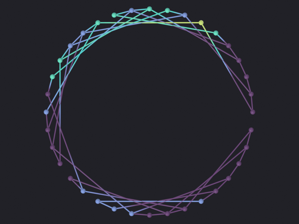
Same style, same camera. The color is edge_crossings, on the EDGE domain, so the ramp lands on the tubes and the node spheres take the per-vertex average of the edges meeting there, a real quantity on the same scale (see sg.render.color_graph): a bright node is a node whose edges all cross something. node_fraction=0.14, lower again than figure 1’s 0.16, because on a circular drawing the tubes carry the measurement.

nb.figure(objects["Grid_convex"],
          "renders/17_topology/3_crossings_convex",
          look='ink', color_attribute="edge_crossings",
          node_fraction=0.14)

  Promoted 1 edge attribute(s) to point domain for GN propagation
Info: Geometry Nodes modifier added
Info: Attribute -> edge_crossings  ·  edge_crossings -> turbo [log]  [0 … 9] on Point

[PASS] 3_crossings_convex.png legible — 6.7% ink (healthy range 0.5–60%)

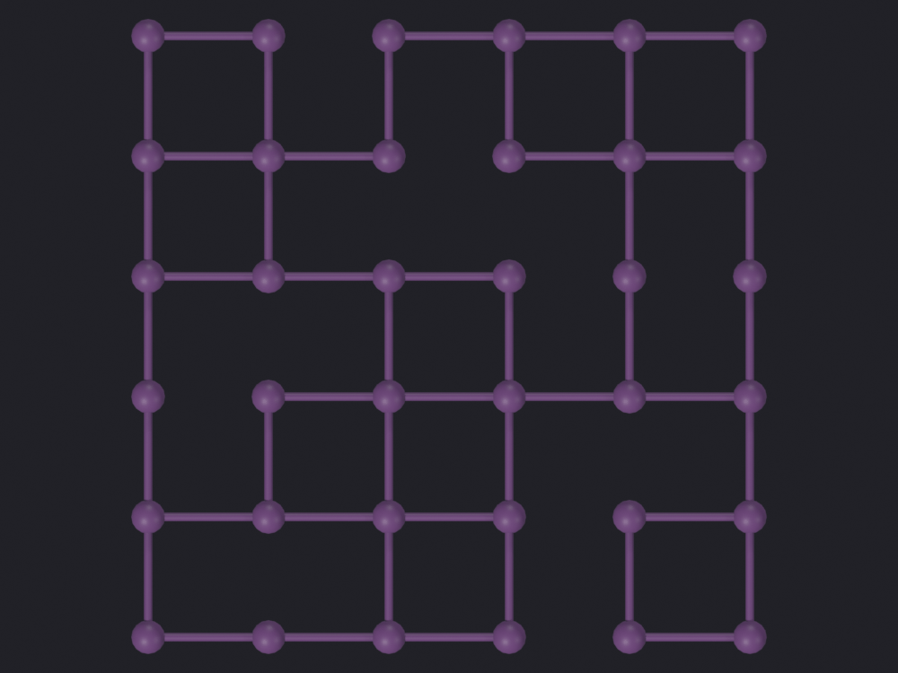
The same 36 nodes and 48 edges put back where the lattice has them. This figure is deliberately one flat color, and that is the result. edge_crossings is 0 on every edge, so the ramp has nothing to span: the coloring reports a range of [0 … 1e-09] and everything lands on turbo’s bottom stop, a dark blue-purple, the weakest color in the look. A constant attribute on a continuous ramp always lands on an endpoint and both of turbo’s endpoints are dark. This figure carries 12 % ink where the convex drawing above carries 7 %, so it is uniform rather than dim, which is what “no edge crosses any other” looks like.

nb.figure(objects["Grid"], "renders/17_topology/4_crossings_free",
          look='ink', color_attribute="edge_crossings",
          node_fraction=0.14)

  Promoted 1 edge attribute(s) to point domain for GN propagation
Info: Geometry Nodes modifier added
Info: Attribute -> edge_crossings  ·  edge_crossings -> turbo [log]  [0 … 1e-09] on Point

[PASS] 4_crossings_free.png legible — 11.6% ink (healthy range 0.5–60%)

When zero is not available

K₅ is not planar, so no drawing of it reaches zero. Its crossing number, the minimum over all drawings, is 1, and the convex drawing measured above is nowhere near it: five crossings, one per C(5,4) quadrilateral.

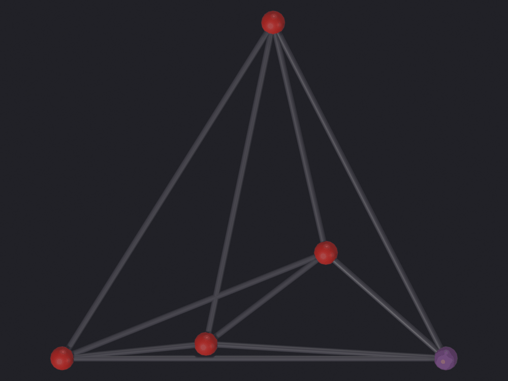
One crossing is reachable with straight lines, and the construction makes the forcing visible. Draw K₄ planar: a triangle A B C with D strictly inside, joined to all three, giving six edges, no crossings and four faces. Add E inside the face A B D, joined to A, B and D without crossing anything. The last edge, E-C, has to leave that triangle, and the only way out crosses one of its three edges.

K5_DRAWING = {0: (-4.0, -2.0),   # A  \
              1: (4.0, -2.0),    # B   } the outer triangle
              2: (0.4, 5.0),     # C  /
              3: (1.5, 0.2),     # D, inside A B C
              4: (-1.0, -1.7)}   # E, inside the face A B D, low and left
best = build(nx.complete_graph(5), K5_DRAWING, "K5_best")
act(best)
with nb.quiet():
    bpy.ops.scigraphs.validate_crossings()
print("K5 convex        : 5 crossings  (C(5,4), measured above)")
print(f"K5 hand-drawn    : {int(best['topo_num_crossings'])} crossing")
print("crossing number of K5, the minimum over every drawing: 1")
check("the hand-drawn K5 achieves the crossing number",
      int(best["topo_num_crossings"]) == 1)
check("but it cannot reach zero, and nothing can",
      int(best["topo_num_crossings"]) >= 1)


Creating graph object with 5 nodes...
  Coordinates applied for 5/5 nodes in 0.00s
  Vertices created in 0.00s
  10 edges created in 0.00s
  Mesh conversion in 0.00s
  Object created in 0.00s
Total graph creation time: 0.00s
Warning: Embedding has 1 edge crossing(s)!
K5 convex        : 5 crossings  (C(5,4), measured above)
K5 hand-drawn    : 1 crossing
crossing number of K5, the minimum over every drawing: 1
[PASS] the hand-drawn K5 achieves the crossing number
[PASS] but it cannot reach zero, and nothing can

True

This figure is colored by a node attribute where the two above it use an edge one. The only way an EDGE-domain attribute reaches a tube is _promote_edge_attributes_to_point, which re-domains it onto the vertices, so Blender averages the edges meeting at each node on the way. On the sparse grid that is harmless. On a five- or six-node complete graph it destroys the figure: K₅ in convex position is vertex-transitive, every vertex meets two 0-crossing edges and two 2-crossing edges, every average is 1, and the render comes back a single flat green with the pentagon and its diagonals indistinguishable. Convex K₃,₃ does the same, with per-edge counts of 0, 2 and 4. Both were rendered and both discarded.

So the measurement moves to the domain that can carry it: which vertices the unavoidable crossing touches. Four of the five, a two-value attribute on turbo’s two dark ends, which the same edge_color of 0.060 answers.

involved = set()
for first, second in topology.detect_edge_crossings_3d(
        [list(v.co) for v in best.data.vertices],
        [(e.vertices[0], e.vertices[1]) for e in best.data.edges],
        tolerance=0.01)["crossing_pairs"]:
    involved |= set(first) | set(second)
flags = [1 if i in involved else 0 for i in range(len(best.data.vertices))]
mesh = best.data
if "in_crossing" in mesh.attributes:
    mesh.attributes.remove(mesh.attributes["in_crossing"])
attr = mesh.attributes.new(name="in_crossing", type='INT', domain='POINT')
attr.data.foreach_set("value", flags)
print("vertices on a crossing edge:", sorted(involved), "of 5")
check("one vertex of the five is not involved", sum(flags) == 4)

nb.figure(best, "renders/17_topology/5_k5_best",
          look='ink', color_attribute="in_crossing",
          node_fraction=0.14, edge_color=LABEL_EDGE_COLOR)

vertices on a crossing edge: [0, 2, 3, 4] of 5
[PASS] one vertex of the five is not involved
Info: Geometry Nodes modifier added
Info: Attribute -> in_crossing  ·  in_crossing -> turbo [log]  [0 … 1] on Point

[PASS] 5_k5_best.png legible — 8.8% ink (healthy range 0.5–60%)

Red: an endpoint of one of the two edges that cross. Purple: B, the one vertex of the five that is not. The single crossing is the X just above E, where the edge E-C leaves the face A B D through A-D. No drawing of this graph has fewer.

Two properties of the detector. topology.detect_edge_crossings_3d compares every pair of edges, O(E²), which is 1,128 pairs for this grid and would be 500,000 for a street network of a thousand edges. It works in 3D, by closest approach between two segments with a distance tolerance the operator fixes at 0.01 Blender units (topology_operators.py:185). On a flat drawing that is a true crossing test, but two edges passing within 0.01 units of each other without touching are counted as a crossing, and 0.01 is not a fraction of the drawing: on a graph imported at scale=0.001, where a neighborhood spans one unit, it is 1 % of the whole scene. Two collinear overlapping segments are missed entirely, because the parallel case returns False at topology.py:642 before any overlap test.

7 · The embedding surface

visualize_surface, labeled Compute Embedding in the UI, does two things, and the second is not what the name suggests.

It recomputes the node positions with nx.planar_layout, the Chrobak-Payne straight-line drawing algorithm, and rebuilds the mesh from them. The result is guaranteed crossing-free.
It adds a child object: a single flat rectangle, sized to the bounding box of the new drawing plus a margin, one hundredth of a unit below it, with a semi-transparent blue material.

That rectangle is the “surface”: a plane, not a torus and not a surface of genus g, and nothing in it depends on anything section 4 computed. There is no path in the add-on from a genus of 1 to a drawing on a torus.

It also requires topo_is_planar on the object already: run without a prior check_planarity it returns “Run planarity check first” rather than running one.

target = objects["Lattice"]
act(target)
before = [a.name for a in target.data.attributes]
print("attributes before:", before)

with nb.quiet():
    bpy.ops.scigraphs.visualize_surface()

surface = bpy.data.objects[target["topo_surface_child"]]
print("attributes after :", [a.name for a in target.data.attributes])
print(f"surface object   : {surface.name}, {len(surface.data.vertices)} verts, "
      f"{len(surface.data.polygons)} face, parent {surface.parent.name}")
print("layout recorded  :", target.get("topo_layout_type"))

act(target)
with nb.quiet():
    bpy.ops.scigraphs.validate_crossings()
print("crossings after the rebuild:", target.get("topo_num_crossings"))

check("the recomputed drawing is crossing-free",
      int(target["topo_num_crossings"]) == 0)
check("the surface is a single quad, not a surface of any genus",
      len(surface.data.polygons) == 1 and len(surface.data.vertices) == 4)
check("the mesh rebuild destroyed every attribute the analysis wrote",
      "face_id" in before and "face_id" not in
      [a.name for a in target.data.attributes])

attributes before: ['position', '.edge_verts', '.corner_vert', '.corner_edge', 'face_id']
Info: Planar embedding - edges DO NOT cross
attributes after : ['position', '.edge_verts', '.corner_vert', '.corner_edge', 'is_intersection']
surface object   : Lattice_Surface, 4 verts, 1 face, parent Lattice
layout recorded  : planar_crossing_free
Info: Embedding is crossing-free!
crossings after the rebuild: 0
[PASS] the recomputed drawing is crossing-free
[PASS] the surface is a single quad, not a surface of any genus
[PASS] the mesh rebuild destroyed every attribute the analysis wrote

True

Operator limitation. _rebuild_graph_mesh replaces obj.data with a freshly built mesh (SciGraphs/ui/operators/scigraphs/topology_operators.py:309) and copies exactly one attribute onto it, is_intersection. Everything else goes: face_id from compute_faces, any centrality, any imported column, any color layer. It also sets num_curve_verts = 0, so a graph whose edges had a curved style comes back straight. Run it before the analysis, or accept that the analysis has to be re-run.

The stale copy the operator leaves behind

A SciGraphs graph carries its node coordinates twice: in the mesh, and in the node_positions custom property the native-graph contract defines. _rebuild_graph_mesh updates num_nodes, num_mesh_verts and num_curve_verts (topology_operators.py:324) and does not update node_positions, so the property still describes the drawing the embedding replaced.

stored = np.asarray(list(target["node_positions"]), dtype=float).reshape(-1, 3)
actual = np.array([list(v.co) for v in target.data.vertices])
spacing_stored = float(np.median(
                       [np.sort(np.linalg.norm(stored - p, axis=1))[1] for p in stored]))
spacing_actual = float(np.median(
                       [np.sort(np.linalg.norm(actual - p, axis=1))[1] for p in actual]))
cloud, source = sg.render.node_cloud(target)
print(f"largest disagreement between property and mesh: "
      f"{np.abs(stored - actual).max():.2f} Blender units")
print(f"median node spacing   property {spacing_stored:.3f}   mesh {spacing_actual:.3f}")
print(f"sg.render.node_cloud reads {source!r}")

check("node_positions still describes the drawing that was replaced",
      not np.allclose(stored, actual))
check("so every radius derived from node spacing comes out far too big",
      spacing_stored / spacing_actual > 5,
      f"{spacing_stored / spacing_actual:.1f}x")

largest disagreement between property and mesh: 8.93 Blender units
median node spacing   property 2.000   mesh 0.227
sg.render.node_cloud reads 'node_positions'
[PASS] node_positions still describes the drawing that was replaced
[PASS] so every radius derived from node spacing comes out far too big — 8.8x

True

Everything that sizes a glyph from node spacing reads that property first (sg.render.node_cloud does, and so does the add-on’s own preview autoscale), so the node radius comes out 8.8 times too large and the figure below would be a row of merged beads. The notebook writes the property back in line with the mesh before rendering.

geometry.update_node_positions_from_property() copies the property onto the mesh, and every layout operator calls it (SciGraphs/ui/operators/scigraphs/data_operators.py:40), so a layout run after visualize_surface writes the old coordinates back over the crossing-free embedding without a word. Demonstrated below on a copy, because it is destructive.

victim = target.copy()
victim.data = target.data.copy()
use_collection().objects.link(victim)
victim.name = "Lattice_Reverted"
geometry.update_node_positions_from_property(victim)
reverted = np.array([list(v.co) for v in victim.data.vertices])
print("after update_node_positions_from_property, the mesh is the old drawing:",
      bool(np.allclose(reverted, stored)))
check("a layout would silently undo the planar embedding",
      np.allclose(reverted, stored))
bpy.data.objects.remove(victim, do_unlink=True)

# So the figure below is sized from the drawing it actually shows.
target["node_positions"] = actual.flatten().tolist()
print("node_positions rewritten from the mesh; median spacing now",
      f"{spacing_actual:.3f}")

after update_node_positions_from_property, the mesh is the old drawing: True
[PASS] a layout would silently undo the planar embedding
node_positions rewritten from the mesh; median spacing now 0.227

The figure

isolate=False so the plate is in the frame with the graph, the only way to see what the operator added. The ceiling of the legibility check is lifted for the reason notebook 13 gives: the plate reaches the corners of the frame, so ink() measures where the plate stops rather than whether the graph reads. The floor still bites.

isolate=False means every mesh in the scene, and by this point the scene holds thirteen graphs on top of one another. Everything but this graph and its plate is handed to hide=, which keeps the framing on the lattice. Without it the frame comes back as all thirteen drawings superimposed, a quiet failure that looks like a render bug rather than a scene-management one.

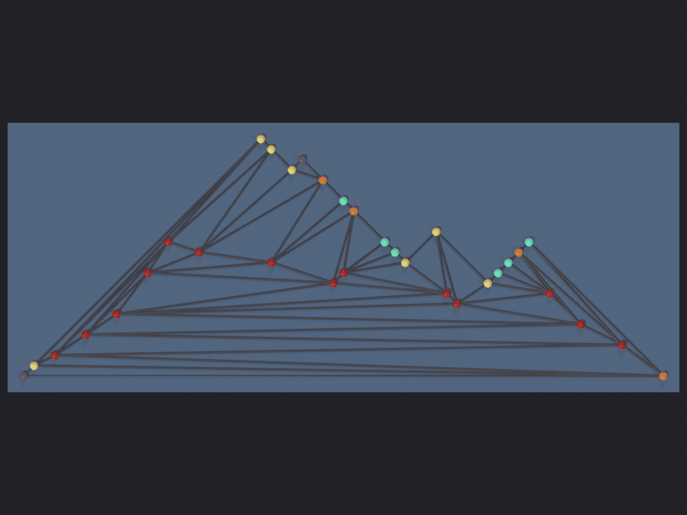
The color is node_degree, computed here because the rebuild took everything else. On the triangular lattice it runs from 2 at the corners to 6 in the interior, so it says where the boundary is, and the boundary is what a planar embedding rearranges most.

The figure is easy to read as a failure and is not one. Chrobak-Payne guarantees a crossing-free straight-line drawing on an integer grid and nothing about how it looks. Every node lands on a lattice of pitch 0.227 units and the whole graph collapses into a wide, shallow wedge, with long chords running almost horizontally underneath it. Compare figure 1, the same kind of object drawn by hand.

degrees = [d for _, d in sorted(lattice.degree())]
mesh = target.data
if "node_degree" in mesh.attributes:
    mesh.attributes.remove(mesh.attributes["node_degree"])
attr = mesh.attributes.new(name="node_degree", type='INT', domain='POINT')
attr.data.foreach_set("value", degrees[:len(mesh.vertices)])
print("degree range:", min(degrees), "-", max(degrees))

crowd = [o for o in bpy.data.objects
         if o.type == 'MESH' and o not in (target, surface)]
path = nb.render(target, "renders/17_topology/6_surface",
                 isolate=False, hide=crowd, look='ink',
                 color_attribute="node_degree",
                 node_fraction=0.30,
                 edge_color=LABEL_EDGE_COLOR, verbose=False)
nb.show(path)
nb.check_render(path, maximum=1.0)

degree range: 2 - 6
  Skipping Split Edges: 'is_intersection' present, keeping streets continuous
Info: Geometry Nodes modifier added
Info: Attribute -> node_degree  ·  node_degree -> turbo [log]  [2 … 6] on Point

[PASS] 6_surface.png legible — 51.4% ink (healthy range 0.5–100%)

True

`toggle_topo_surface` and `remove_topo_surface`

The same pair as for the dual, reading topo_surface_child off the active object. remove is the one that matters under a live kernel: the plate is a real object in the scene and every later isolate=False render composes against it.

act(target)
with nb.quiet():
    bpy.ops.scigraphs.toggle_topo_surface()
print("surface hidden:", surface.hide_viewport)
with nb.quiet():
    bpy.ops.scigraphs.toggle_topo_surface()
check("toggling the surface twice is the identity", not surface.hide_viewport)

Info: Surface hidden
surface hidden: True
Info: Surface visible
[PASS] toggling the surface twice is the identity

True

8 · Cleaning up after the operators

create_dual_graph and visualize_surface leave objects behind, and under the single shared kernel these notebooks run in, that state is still there when the next notebook starts. Both have a remove_* operator; the plain graphs are ours to clear.

for name, obj in list(objects.items()):
    if obj.get("topo_dual_child"):
        act(obj)
        with nb.quiet():
            bpy.ops.scigraphs.remove_dual_graph()
    if obj.get("topo_surface_child"):
        act(obj)
        with nb.quiet():
            bpy.ops.scigraphs.remove_topo_surface()

leftover = [o.name for o in bpy.data.objects
            if o.name.endswith("_Dual") or o.name.endswith("_Surface")]
print("dual / surface objects left in the scene:", leftover or "none")
check("the operators' side objects are gone", not leftover)
check("the keys that pointed at them are gone",
      not any(o.get("topo_dual_child") or o.get("topo_surface_child")
      for o in bpy.data.objects))

Info: Dual graph removed
Info: Surface removed
dual / surface objects left in the scene: none
[PASS] the operators' side objects are gone
[PASS] the keys that pointed at them are gone

True

9 · Save

Every graph, what the operators said, and what the answer is.

output_dir = nb.out("05_topology")
output_dir.mkdir(parents=True, exist_ok=True)

rows = ["graph,V,E,known_planar,operator_planar,F,chi,genus_bound,known_genus"]
for name, graph, _positions, planar in CAST:
    obj = objects[name]
    rows.append(",".join(str(x) for x in (
                name, graph.number_of_nodes(), graph.number_of_edges(),
                planar, verdicts[name],
                obj.get("topo_num_faces", ""), obj.get("topo_euler_chi", ""),
                obj.get("topo_genus_lower_bound", ""),
                GENUS_KNOWN.get(name, ""))))
(output_dir / "topology_cases.csv").write_text("\n".join(rows) + "\n",
                                               encoding="utf-8")

faces_rows = ["face_id,degree,nodes"]
for index, face in enumerate(faces):
    faces_rows.append(f"{index},{len(face)},\"{' '.join(str(v) for v in face)}\"")
(output_dir / "grid_faces.csv").write_text("\n".join(faces_rows) + "\n",
                                           encoding="utf-8")

print("written to", nb.rel(output_dir))
for entry in sorted(output_dir.iterdir()):
    print("  ", entry.name, f"{entry.stat().st_size / 1e3:.1f} kB")

written to notebooks/out/05_topology
   grid_faces.csv 0.4 kB
   topology_cases.csv 0.5 kB

Rendering

Six figures, all EEVEE through nb.figure() / render_eevee(), all look='ink' on turbo, all straight down through an orthographic camera: the suite’s style since notebook 13, so these plane graphs read the same way as the street networks in 01 and 05.

What this notebook had to solve that the others did not: its attributes are categorical or binary, and turbo is neither. Hence the measured ramp separations, the clipping, the neutral at (0.060, 0.056, 0.071), and node sizes derived from each drawing rather than left at the 0.35 default.

Two figures were made and thrown away: convex K₅ and convex K₃,₃ colored by edge_crossings both render as one flat color. The weakest figure that survived is figure 2, the dual, where the outer face’s vertex is placed 15 % of the median spacing from its nearest neighbor and half disappears behind it. No render setting fixes that; the operator put it there.

The Vulkan warning that applies to the SciGraphs GPU engine applies here too if you switch to it: gpu.state.point_size_set is a no-op for the add-on’s shaders on Vulkan, the Linux default, so POINT and DISK nodes rasterize one pixel wide. Start Blender with --gpu-backend opengl.

Summary

Operator	Verified against
`check_planarity`	the literature, 13/13 correct
`compute_faces`	V − E + F = 2 on five connected planar graphs; Σ deg(f) = 2E; F = 1 for a tree
`calculate_genus`	exact 0 when planar; a lower bound otherwise, tight on K₅, K₇, K₈
`create_dual_graph`	V* = F ✓; E* < E ✗
`validate_crossings`	an interleaving oracle, which gives C(n,4) on convex K₄, K₅, K₆
`visualize_surface`	0 crossings after the rebuild

Six things measured here that are not written down anywhere else.

calculate_genus reports Genus >= 0 for two graphs it has just declared non-planar (§4, topology.py:307).
The Kuratowski classifier is dead code (§2, topology.py:356).
The geometric dual is the simple dual: a 48-edge grid yields a 29-edge dual of which 28 reach the mesh, with the outer face’s vertex at the mean of the perimeter (§5, topology.py:246, topology_operators.py:468).
Euler’s identity holds in the form χ = 2C, and an edgeless component contributes no face at all (§3, topology.py:62).
visualize_surface leaves node_positions describing the drawing it just replaced: the two copies disagree by up to 8.9 Blender units, 2.000 median spacing against the mesh’s 0.227, so every radius derived from spacing comes out 8.8x too large, and a later layout copies the stale property back over the embedding (§7, topology_operators.py:324, data_operators.py:40).
A crossing count does not survive a layout: rebuild_edges zeroes every EDGE-domain attribute (§6, geometry.py:1226).

validate_crossings is not on that list: C(n,4) for convex K₄, K₅ and K₆, the same answer as an independent interleaving count on convex K₃,₃, 78 for the grid drawn on a circle and 0 for the same graph drawn as a lattice. That number is about the drawing, and moving it is 16 · Layouts’ job.